Thinned Mean Field Langevin Dynamics
Abstract: Several important learning tasks can be formulated as minimizing an entropy-regularized objective over an appropriate space of probability distributions. Mean-field Langevin dynamics (MFLD) facilitate computation in this general context, casting the minimizer as the invariant distribution of a McKean--Vlasov process, which can be numerically discretized using $N$ particles and thus simulated. However, simulating this interacting particle system has computational complexity of order $N2$. Motivated by recent research into \emph{kernel thinning}, we propose \texttt{KT-MFLD}, in which each particle interacts only with a thinned particle coreset of size $\mathcal{O}(N{\frac{1}{2}})$. \texttt{KT-MFLD} thus reduces the computational complexity to order $N{\frac{3}{2}}$ while, under mild regularity conditions, achieving the same convergence guarantees (up to logarithmic factors) as MFLD. Our theoretical analysis is empirically confirmed on tasks including the training of student-teacher neural networks, quantization with maximum mean discrepancy, and computation of predictively-oriented posteriors in a post-Bayesian framework.

Paper Prompts
Sign up for free to create and run prompts on this paper using GPT-5.
Top Community Prompts
Explain it Like I'm 14
Thinned Mean Field Langevin Dynamics — A Simple Explanation
Overview: What is this paper about?
This paper is about making a popular but expensive machine learning method much faster without losing much accuracy. The method, called mean-field Langevin dynamics (MFLD), uses lots of tiny “particles” (think: dots on a screen) that move around with a mix of push-and-pull forces and a bit of randomness. Over time, the particles settle into a shape that represents the best answer to a learning problem. The problem is: with N particles, the usual way costs about O(N2) work each step because every particle talks to every other particle.
The paper introduces a faster version, KT-MFLD, where each particle only talks to a small, smartly chosen set of about √N “representative” particles. This cuts the work to about O(N{3/2}) per step and still keeps the same guarantees (up to some small extra “log” factors).
The goals in simple terms
The authors aim to:
- Speed up MFLD so it can handle many more particles and bigger problems.
- Keep the method accurate and reliable.
- Prove mathematically that the faster method still converges to the right answer.
- Show it works well in practice on several tasks (training neural nets, compressing distributions, and robust statistical inference).
How the method works (with everyday analogies)
Here are the key ideas, explained simply:
- Distributions and particles: Many ML problems ask for the “best distribution” over answers (a smart way to represent uncertainty). MFLD represents this distribution with many particles (little dots). If the dots spread out just right, they match the target distribution.
- Entropy regularization: “Entropy” measures how spread-out the distribution is. Adding entropy acts like a “don’t overfit” rule: it encourages solutions that aren’t too spiky, similar to how a teacher might prefer homework that’s neat and balanced instead of crammed into one corner.
- Langevin dynamics: Each particle is nudged by forces that pull it toward better places (like rolling downhill on a landscape shaped by the learning objective) plus a bit of random jiggle (like thermal noise). Over time, the crowd of particles settles into the desired distribution.
- Why it’s slow: In classic MFLD, each particle looks at all other particles to figure out its next move. That’s like a classroom where every student has to talk to every other student before deciding what to do—very slow!
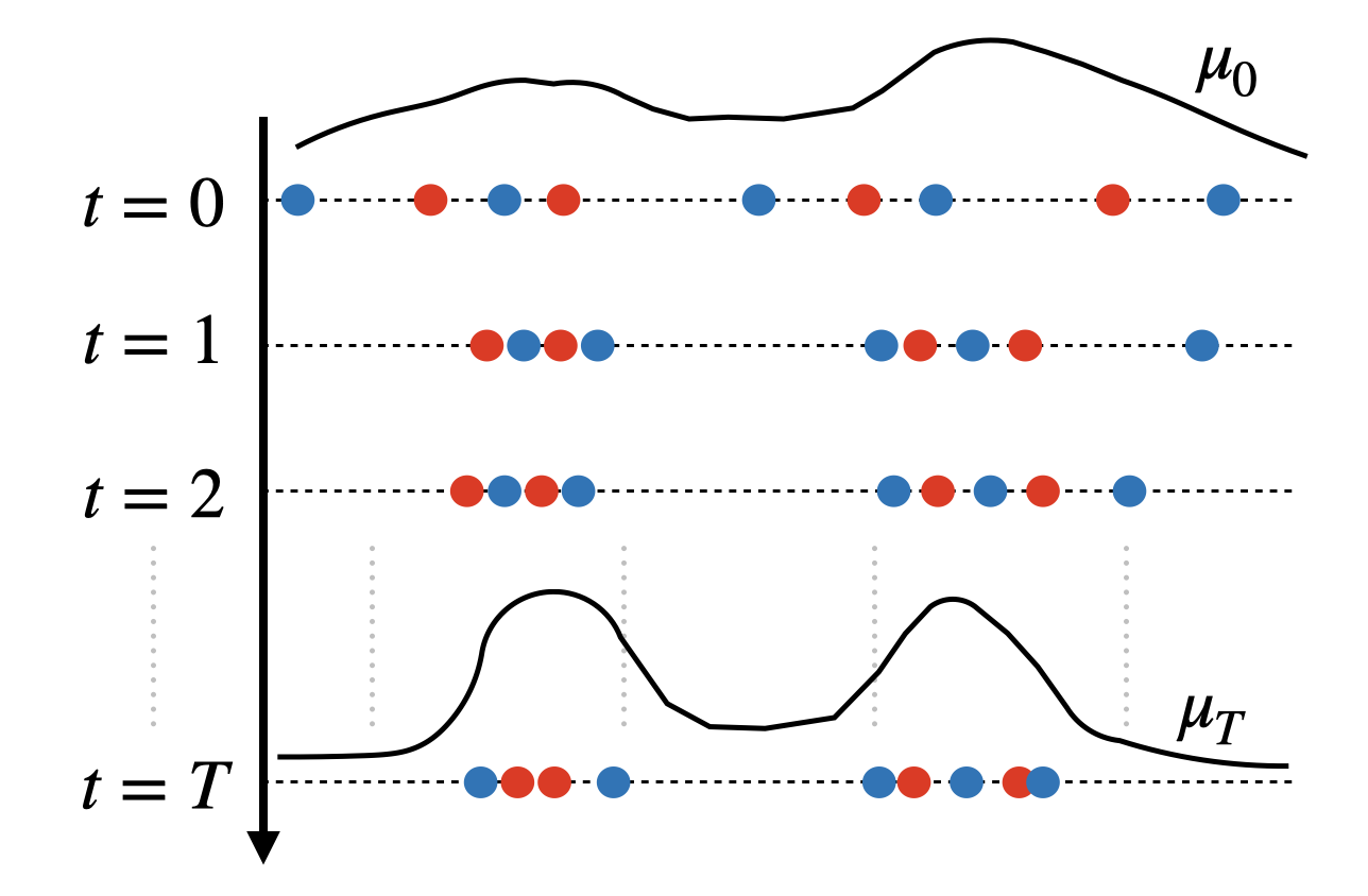
- Kernel thinning (the big trick): Instead of talking to everyone, each step picks about √N “class representatives” using a clever method called kernel thinning (the paper uses a near-linear-time algorithm named kt-split; they also try KT-Compress). Now every student only talks to the reps. This keeps the group’s overall opinion accurate but saves a lot of time.
- Coreset: The small set of representatives is called a “coreset.” It’s chosen so that averaging over the coreset is almost as good as averaging over all particles.
- Cost comparison:
- Before: O(N2) per step (everyone talks to everyone).
- After: O(N{3/2}) per step (everyone talks to about √N reps), plus a small overhead to pick the reps.
Main results and why they matter
What the authors prove and show:
- Nearly the same accuracy as the original: They prove that KT-MFLD converges to the right answer with error that shrinks like about 1/N (up to some logarithmic factors), which matches the original MFLD’s rate in the important “number of particles” term. In contrast, simple random subsampling loses much more accuracy, only shrinking like 1/√N.
- Much faster per step: Switching from O(N2) to O(N{3/2}) means you can afford many more particles or steps in the same compute time. More particles usually means a better approximation of complex, multi-peaked distributions.
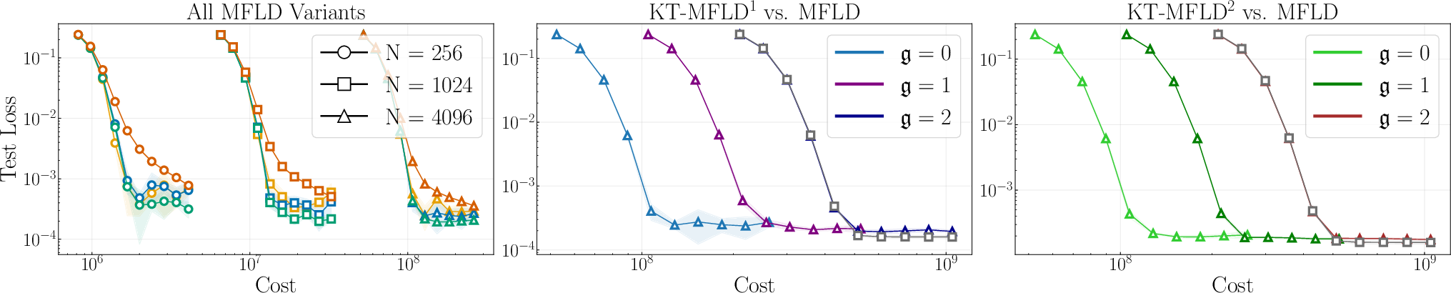
- Stronger than random thinning and random batching: In experiments, KT-MFLD consistently beats:
- Random-MFLD (randomly picking the √N reps),
- RBM-MFLD (dividing particles into random batches),
- because kernel thinning chooses a better coreset than simply picking randomly.
- Works on several tasks:
- Training a student neural network from a teacher (mean-field neural nets),
- Compressing a distribution (quantization) using maximum mean discrepancy (MMD),
- Predictively-oriented posteriors (a robust alternative to standard Bayesian inference) in a misspecified predator–prey model.
Across these, KT-MFLD delivers better results for the same computational budget. In some tasks, the KT-Compress variant shines because it aligns especially well with MMD goals; in others, kt-split performs best. Both are strong.
- Practical takeaway: For the same amount of computing time, KT-MFLD often matches or beats the original MFLD because you can run more particles or more steps.
Why this is important
- Scalability: Many modern problems need thousands of particles to capture complicated shapes (think: many modes/peaks). Cutting the per-step cost lets you use bigger particle sets and get better answers.
- Reliability with theory: The method isn’t just a heuristic; it comes with proofs that it converges and matches the accuracy of the original approach (up to small log factors), unlike naive subsampling.
- Broad usefulness: The technique helps in:
- Training certain wide neural networks more efficiently,
- Building small, high-quality summaries of big distributions (coresets),
- Doing robust inference when your model is imperfect (common in real-world science).
Final thoughts: Impact and future directions
KT-MFLD shows how to use smart, theory-backed thinning to make powerful but costly particle methods practical at larger scales. This can open the door to:
- Better uncertainty modeling in complex systems,
- Faster training for mean-field-style neural models,
- More robust statistical inference in scientific problems where the model is only an approximation.
The idea—use a high-quality coreset each step—could also accelerate other particle-based algorithms beyond MFLD, making them more feasible for real-world, large-scale applications.
Knowledge Gaps
Knowledge gaps, limitations, and open questions
Below is a concise list of unresolved issues, limitations, and open questions that emerge from the paper’s assumptions, theory, algorithms, and experiments. These can guide future research.
- Restrictive RKHS assumptions and practical mismatch:
- The theory requires q₁(u,·) ∈ H_k and ∇₁q₂(x,·) ∈ H_k{⊗d} under a bounded kernel k, but in mean-field neural networks this may require an empirical kernel over the full dataset, which is computationally prohibitive; in experiments, different (Sobolev) kernels are used. A principled, computationally feasible way to select k that certifiably matches the function class driving the vector field is not provided.
- KT-Compress theoretical gap:
- KT-Compress guarantees rely on a uniform-in-time bound on max_i ||x_t{(i)}||; the paper notes it is unclear whether such a bound holds for MFLD. Establishing uniform moment/compactness bounds for particle trajectories to justify KT-Compress in theory remains open.
- Dimension dependence and curse of dimensionality:
- The bound includes ᾱ in the denominator of the thinning-induced error term, and ᾱ can be exponentially small in dimension d. Dimension-free or dimension-robust guarantees (or alternative analyses that avoid exponential dependence) are not provided.
- Optimal coreset size and oversampling:
- The choice M ≍ √N is adopted from thinning theory, with an oversampling parameter 𝔤 to remove log factors, but there is no analysis of whether √N is optimal under a given compute budget or problem structure. Optimal scaling of M (and 𝔤) as functions of N, d, σ, γ, and task-dependent constants is not established.
- Thinning frequency and staleness:
- The algorithm thins at every iteration. It is unknown how thinning less frequently (e.g., every k steps), or maintaining/refreshing coresets adaptively, affects accuracy and total cost. Theory for thinning frequency and coreset refresh policies is missing.
- Uniform-in-time and function-class uniformity:
- The thinning bound used (for kt-split) controls integration error for a fixed f with probability 1−δ. The vector field depends on μ (and hence the coreset) and changes over time and across particles. Uniform (in t, i) control over a relevant function class, and a choice of δ that accounts for T iterations, is not developed.
- Convergence metric and practical distances:
- The main result bounds (σ/N) KL(μT{(N)} || π{⊗N}); a finite-time, finite-N bound in metrics directly tied to the empirical distribution (e.g., W₂(μ{X_T}, π)) or to task-specific losses (e.g., MMD or KGD) is not derived.
- Nonconvex objectives:
- The analysis requires convexity of F₀ in the space of measures. Many practical objectives (e.g., more general neural architectures) are nonconvex; extensions of KT-MFLD guarantees to nonconvex mean-field objectives are open.
- Small-noise limit:
- Guarantees assume σ>0 due to entropy regularization; the behavior as σ→0 (vanishing-noise limit) and the impact on required N, M, T, and γ are not analyzed.
- Kernel selection and hyperparameter tuning:
- Performance of kernel thinning depends critically on kernel choice (e.g., lengthscale) and can degrade in high dimensions. There is no guidance for selecting/tuning k to match q₁, q₂ (or their gradients), nor an analysis of sensitivity to kernel misspecification.
- Weighted coresets:
- The method uses uniformly weighted coreset points; whether weighted thinning (importance-weighted or quadrature-weighted coresets) could reduce drift bias and improve accuracy is not studied.
- Interaction cost beyond pairwise terms:
- For applications where evaluating q₁/q₂ is costly (e.g., PrO posteriors that involve ODE solves), the end-to-end complexity may be dominated by model solves rather than pairwise interactions. A refined complexity/error analysis that accounts for model-solve costs is absent.
- Approximation of E_{u∼ρ}:
- In settings where the expectation over u∼ρ is approximated via Monte Carlo, the joint effect of thinning error and Monte Carlo error (variance/bias) is not analyzed, nor is guidance given on inner sample sizes.
- Step-size schedules and adaptivity:
- Theory assumes a fixed small γ with conservative bounds; there is no analysis of optimal γ choices, decreasing schedules, or adaptive step-size/variance strategies for KT-MFLD.
- Propagation of chaos and fluctuation analysis:
- How thinning affects propagation-of-chaos properties, finite-N fluctuations, and long-time stability of the particle system is not addressed.
- Long-time/ergodic behavior:
- Theoretical bounds are stated for fixed T; uniform-in-T (ergodic) guarantees and mixing-time analyses for thinned dynamics are not provided.
- Extensions to other interacting particle systems:
- The paper asserts applicability to SVGD and kernel gradient flows but does not develop the corresponding theory or provide guarantees in those settings.
- Unbounded kernels and heavy-tailed targets:
- Assumptions require bounded kernels and bounded derivatives of q₁/q₂. Extensions to unbounded kernels (e.g., polynomial kernels) and heavy-tailed targets are not covered.
- Additional linear terms and latent-variable costs:
- Linear terms ∫q₃(x)dμ(x) are omitted as “only O(N)” to compute; however, in some tasks q₃ may involve latent integrals or expensive evaluations. Thinning or approximation strategies for such terms are not analyzed.
- Parallel and distributed scalability:
- kt-split requires a global pass over particles each iteration; parallel/distributed implementations and their synchronization/communication costs are not discussed, in contrast to naturally parallel batch methods.
- Constant sizes and practical tightness:
- Important constants (B, c₀, C₃, ᾱ) are unspecified and may be large in practice, potentially making the bounds loose. Problem-dependent estimates or empirical calibration of these constants are not given.
- High-dimensional kernel thinning:
- Beyond ᾱ’s dependence, kernel thinning itself may suffer from concentration in high d (e.g., κ = sup_x k(x,x) and RKHS norm growth). Dimension-adaptive kernels or feature maps to mitigate this are not explored.
- Choice of M beyond √N across tasks:
- Empirical results vary (e.g., KT-Compress outperforming kt-split in MMD quantization). A task-adaptive prescription for M (and algorithm choice) balancing error and cost is not provided.
- Theoretical support for experimental kernel choices:
- In neural network and PrO experiments, Sobolev kernels are used for thinning; the paper does not verify that q₁ and ∇q₂ lie in the associated RKHS with controlled norms, leaving a gap between assumptions and practice.
- State-space generality:
- The analysis focuses on ℝd. Extensions to manifolds or constrained domains (and corresponding thinning kernels and guarantees) are not discussed.
Practical Applications
Immediate Applications
The following items outline concrete, deployable use cases that can adopt KT‑MFLD (kernel‑thinned mean‑field Langevin dynamics) now, with suggested workflows and caveats.
- Accelerated training of wide two‑layer mean‑field neural networks (sectors: software/AI, academia)
- What: Replace standard MFLD with KT‑MFLD during noisy gradient descent on wide two‑layer networks to cut per‑iteration cost from O(N²) to O(N{3/2}), enabling larger particle counts N for a fixed compute budget and improved generalization (as observed in student–teacher experiments).
- How: At each iteration, run kt‑split to select a coreset of size M≈⌈√N⌉ (optionally oversample via 𝔤≥0), compute the drift using only the coreset (Eq. 10 in the paper), and update all N particles with Euler–Maruyama.
- Tools/products: A PyTorch/JAX optimizer plugin “KT‑MFLD” with kt‑split or KT‑Compress backends; support for Sobolev/RBF kernels; batch‑wise online learning integration.
- Assumptions/dependencies: Smoothly clipped activations and convex Lipschitz losses (Assumption 1); access to a bounded kernel k such that q₁(u,·)∈H_k (Assumption 2); step‑size tuning γ and noise σ; performance depends on kernel choice and may degrade in very high dimensions.
- Faster MMD‑based dataset quantization and generator training (sectors: software/AI, data engineering, academia)
- What: Use KT‑MFLD (preferably with KT‑Compress) to minimize MMD for dataset summarization, kernel herding–style coreset construction, or training generator networks with MMD losses, achieving better MMD for the same compute vs. random thinning or random batching.
- How: Optimize particle locations to minimize MMD to a target distribution; thin with KT‑Compress (strong MMD guarantees) at each step; deploy larger N under the same time budget.
- Tools/products: “KT‑MMD Quantizer” for dataset compression and fast generative modeling; integration with existing MMD toolkits (e.g., GPyTorch, KeOps).
- Assumptions/dependencies: Bounded, smooth kernel κ (e.g., Gaussian, sufficiently smooth Matérn); the kernel used for thinning should align with the MMD objective; curse‑of‑dimensionality can affect constants; careful selection of coreset size M and oversampling 𝔤.
- Practical PrO (Predictively‑Oriented) posterior inference for mechanistic models (sectors: healthcare, scientific computing, public policy, academia)
- What: Make robust, post‑Bayesian predictive inference feasible for misspecified mechanistic models (e.g., Lotka–Volterra, SIR epidemics) by reducing the O(N²) cost of particle interactions—critical when each interaction requires solving ODEs/PDEs.
- How: Formulate PrO objective with kernel scoring rules; run KT‑MFLD to update N particles while evaluating drifts only against a thinned coreset each iteration; parallelize model solves across particles.
- Tools/products: A “PrO‑inference” module with KT‑MFLD for ODE/PDE‑based models (SciPy/torchdiffeq backends); dashboards for model calibration and robust forecasting.
- Assumptions/dependencies: Bounded kernels on prediction space; differentiable simulators with bounded gradients/Hessians in parameters; compute budget dominated by forward solves; kernel choice and dimensionality affect thinning error; uncertainty in σ, γ tuning.
- Accelerated kernel quadrature and Bayesian cubature node optimization (sectors: scientific computing, finance, energy, academia)
- What: Use KT‑MFLD to optimize node sets that minimize kernel discrepancies to target measures, speeding up Bayesian cubature/Kernel Stein discrepancies for uncertainty quantification and model evidence approximation.
- How: Define F as MMD or kernel discrepancy; thin nodes via kt‑split each iteration to compute drifts efficiently; iterate to strong node sets under fixed compute.
- Tools/products: “KT‑Cubature” library for fast node optimization; integration with probabilistic numerics frameworks.
- Assumptions/dependencies: Same kernel regularity as MMD; target measures and kernels chosen to keep gradients bounded; performance may suffer with extremely high‑dimensional integrands.
- Thinning‑augmented particle optimization methods (e.g., SVGD, kernel gradient descent) (sectors: software/AI, academia)
- What: Apply the same thinning workflow to other interacting particle methods that use pairwise kernel interactions, reducing per‑step costs without redesigning the optimizer.
- How: Swap full pairwise interactions for coreset‑based interactions at each step; reuse kt‑split/KT‑Compress tooling.
- Tools/products: “KT‑SVGD” and “KT‑KGD” variants in existing libraries (e.g., PyTorch SVGD, JAX implementations).
- Assumptions/dependencies: Requires kernels and drift terms to admit the same boundedness/Lipschitz properties; theoretical guarantees may be weaker than for KT‑MFLD until analyzed for each method.
- Resource‑constrained or on‑device probabilistic updating (sectors: mobile/edge AI, embedded systems)
- What: Maintain larger particle sets for personalization or adaptive filters under tight compute/memory constraints by thinning interactions each update.
- How: Deploy KT‑MFLD with small M, tuned γ and σ; run on‑device with periodic re‑thinning.
- Tools/products: Edge inference SDKs incorporating thinning routines; lightweight kt‑split implementations.
- Assumptions/dependencies: Small memory footprint kt‑split; stability requires careful kernel and step‑size choices; benefits taper in very high‑dimensional parameter spaces.
Long‑Term Applications
These opportunities are promising but need additional research, scaling, or engineering before production use.
- High‑dimensional, dimension‑robust thinning and guarantees (sectors: software/AI, finance, healthcare, academia)
- Opportunity: Address the curse‑of‑dimensionality in the thinning‑induced error term (via 𝛼̄ in the bound) with dimension‑adaptive kernels, projections, or preconditioned dynamics.
- Potential products: Auto‑tuned kernel/thinning modules that learn low‑dimensional structure on the fly.
- Dependencies: New theory for dimension‑free/robust rates; scalable estimators of structure (e.g., random features, score preconditioning).
- Deep mean‑field models beyond two layers (sectors: software/AI, academia)
- Opportunity: Extend KT‑MFLD to multi‑layer mean‑field limits and implicit distribution objectives arising in deep architectures.
- Potential products: “KT‑MFLD‑Deep” training engines; integration into large‑scale training pipelines.
- Dependencies: Generalizing first‑variation structure and regularity assumptions to deep settings; empirical validation and convergence theory.
- Streaming/online thinning and distributed/asynchronous implementations (sectors: software/AI, cloud computing)
- Opportunity: Develop incremental kt‑split/KT‑Compress for streaming particle sets and asynchronous distributed training.
- Potential products: Cloud services offering KT‑MFLD as a managed, distributed optimizer; GPU/TPU‑friendly thinning kernels.
- Dependencies: Algorithms for incremental coresets with theoretical guarantees; robust parallelization and communication‑efficient protocols.
- Policy‑facing robust forecasting under model misspecification (sectors: public policy, health, climate/energy)
- Opportunity: Use PrO posteriors computed via KT‑MFLD for policy‑relevant forecasting (epidemics, ecological management, energy demand), where robustness to misspecification is crucial.
- Potential products: Decision‑support tools with PrO‑based uncertainty; scenario exploration dashboards.
- Dependencies: Validation on real‑world policy datasets; stakeholder‑appropriate interpretability; governance and auditability of kernels and objectives.
- Mean‑field games and PDE‑constrained control (sectors: robotics, operations research, energy)
- Opportunity: Apply thinning to particle methods for mean‑field games/control where pairwise interactions dominate compute.
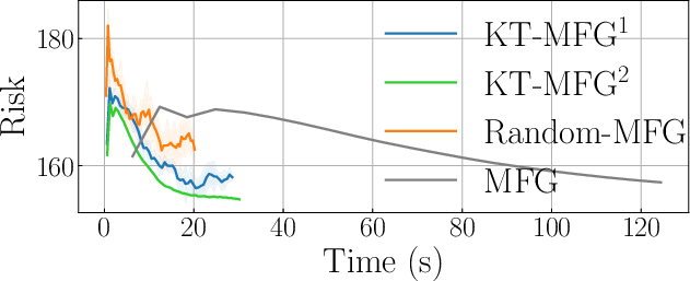
- Potential products: “KT‑MFG” solver modules for planning/control in large populations.
- Dependencies: Extending theory to specific interacting dynamics and verifying stability/accuracy under thinning; specialized kernels tied to game/PDE structure.
- Hybrid fast‑interaction stacks (sectors: software/AI, HPC)
- Opportunity: Combine thinning with other accelerations (e.g., neighbor lists, low‑rank/fast multipole approximations, random features) for sub‑O(N{3/2}) effective costs.
- Potential products: Auto‑selector that switches among thinning, RBM, and low‑rank schemes based on runtime diagnostics.
- Dependencies: Robust estimators of interaction structure; convergence proofs under hybridization.
- Auto‑kernel selection and hyperparameter governance (sectors: software/AI, compliance)
- Opportunity: Automate selection of kernels (for both objective and thinning), coreset size M, and oversampling 𝔤 with performance guarantees.
- Potential products: Hyperparameter auto‑tuning with uncertainty estimates and guardrails.
- Dependencies: Meta‑learning or cross‑validation under implicit objectives; monitoring for stability and fairness across tasks.
Common assumptions and dependencies across applications
- Regularity conditions: Boundedness/Lipschitzness of q₁, q₂, and their derivatives; convexity/Lipschitz derivative of R₁; membership of q₁(u,·) and ∇q₂(x,·) in an RKHS with bounded kernel (Assumptions 1–2).
- Kernel choices: Thinning quality and theory depend on using appropriate bounded kernels (e.g., Gaussian, smooth Matérn, Sobolev). Mismatch between thinning kernel and objective can reduce gains.
- Dimensionality: The thinning‑induced error includes terms that may scale poorly with dimension (via 𝛼̄). High‑d settings may require preconditioning or dimension reduction.
- Algorithmic knobs: Step size γ, noise σ, regularization ζ, coreset size M≈⌈√N⌉, and oversampling 𝔤 affect both accuracy and compute; small γ improves discretization error but increases iterations.
- Compute profile: kt‑split/KT‑Compress are near‑linear per iteration and typically dominated by drift evaluations; in simulator‑based inference, forward model solves dominate cost even after thinning.
Glossary
- Brownian motion: A continuous-time stochastic process with independent Gaussian increments used to model random fluctuations. "and is a standard Brownian motion on ."
- Coreset: A small, representative subset of points that approximates the full set for downstream computations. "The quality of the thinned coreset is evaluated by the integration error"
- Differential entropy: A continuous analogue of entropy measuring uncertainty of a continuous random variable’s distribution. "denotes the differential entropy"
- Empirical measure: The discrete probability measure that places equal mass on each sample/particle. "empirical measure $\mu_{X_s}=\frac{1}{N} \sum_{i=1}^N \delta_{#1{x}_s^{(i)}$"
- Euler–Maruyama method: A numerical scheme for simulating stochastic differential equations via time discretization. "for example using the Euler--Maruyama method"
- First variation: The functional derivative describing the infinitesimal change of a functional with respect to perturbations of a measure. "$F'[\mu_s]:R^d\toR$ is the first variation of at "
- Hessian: The matrix of second-order partial derivatives of a function. "$H_1 q(#1{x}, #1{x}^{\prime}) \in R^{d\times d}$ (resp $H_2 q(#1{x}, #1{x}^{\prime})$) as the Hessian"
- Invariant distribution: A probability distribution that remains unchanged under the dynamics of a stochastic process. "casting the minimizer as the invariant distribution of a McKean--Vlasov process"
- Kernel gradient discrepancy (KGD): A discrepancy measure tailored to objectives defined via kernelized gradients. "an evaluation metric called kernel gradient discrepancy (KGD)"
- Kernel scoring rule: A strictly proper scoring rule based on kernels to compare predictive distributions. "or the kernel scoring rule "
- Kernel thinning: A technique to subsample points using kernel methods while controlling integration error in an RKHS. "Kernel thinning aims to thin (i.e., subsample) a sequence of points"
- KL divergence: A non-symmetric measure of difference between two probability distributions. ""
- KT-Compress: A near-linear-time kernel-thinning algorithm with MMD guarantees under certain conditions. "KT-Compress"
- kt-split: A near-linear-time kernel-thinning algorithm used to build representative subsets. "called kt-split \citep{shetty2021distribution}"
- Langevin dynamics: A stochastic process combining gradient descent with Gaussian noise to sample from target distributions. "we recover Langevin dynamics, which can be simulated using a single particle"
- Law (of a random variable): The probability distribution of a random variable. ""
- Lipschitz continuity: A smoothness condition where the difference of function values is bounded by a constant times the input distance. "is -Lipschitz"
- Lotka–Volterra model: A pair of differential equations modeling predator–prey population dynamics. "LotkaâVolterra model"
- Maximum mean discrepancy (MMD): A kernel-based distance between probability distributions defined via RKHS embeddings. "squared maximum mean discrepancy (MMD)"
- McKean–Vlasov process: An SDE whose drift depends on the distribution of the process itself. "a McKean--Vlasov process"
- Positive definite (kernel): A kernel whose associated Gram matrices are positive semidefinite and strictly positive definite under conditions, ensuring a valid RKHS. "and positive definite"
- Positive semi-definite kernel: A kernel function whose Gram matrices are positive semidefinite for any finite set of inputs. "symmetric positive semi-definite kernel"
- Product measure: The joint measure formed by independent copies of a distribution across multiple dimensions or particles. "for the -fold product measure."
- Proper scoring rule: A scoring function for probabilistic predictions that is minimized only by the true distribution. "a proper scoring rule "
- Random batch method (RBM): An acceleration technique for interacting particle systems that randomly partitions particles into batches each iteration. "random batch method (RBM-MFLD)"
- Reproducing Kernel Hilbert Space (RKHS): A Hilbert space of functions with the reproducing property associated with a kernel. "reproducing kernel Hilbert space (RKHS) "
- Sobolev kernel: A kernel associated with Sobolev spaces that controls function smoothness via derivatives. "we instead use a Sobolev kernel for both versions of KT-MFLD in our experiments."
- Spectral/operator norm: The largest singular value of a matrix, measuring its maximum stretching factor. " denotes its spectral/operator norm."
- Stein variational gradient descent: A deterministic particle method for approximate inference using Stein’s identity and kernelized gradients. "Stein variational gradient descent"
- Stochastic differential equation (SDE): A differential equation driven by stochastic processes like Brownian motion. "stochastic differential equation: given an initial distribution"
- Tensor product: The construction combining spaces to represent multi-dimensional linear mappings or function outputs. "for its -fold tensor product."
- Thinning: The process of selecting a representative subset of particles to reduce computational cost. "We refer to this selection procedure as thinning."
- Wasserstein-2 metric: A distance between probability measures based on optimal transport with quadratic cost. "with respect to the Wasserstein-2 metric"
Collections
Sign up for free to add this paper to one or more collections.

