Hybrid Neural World Models
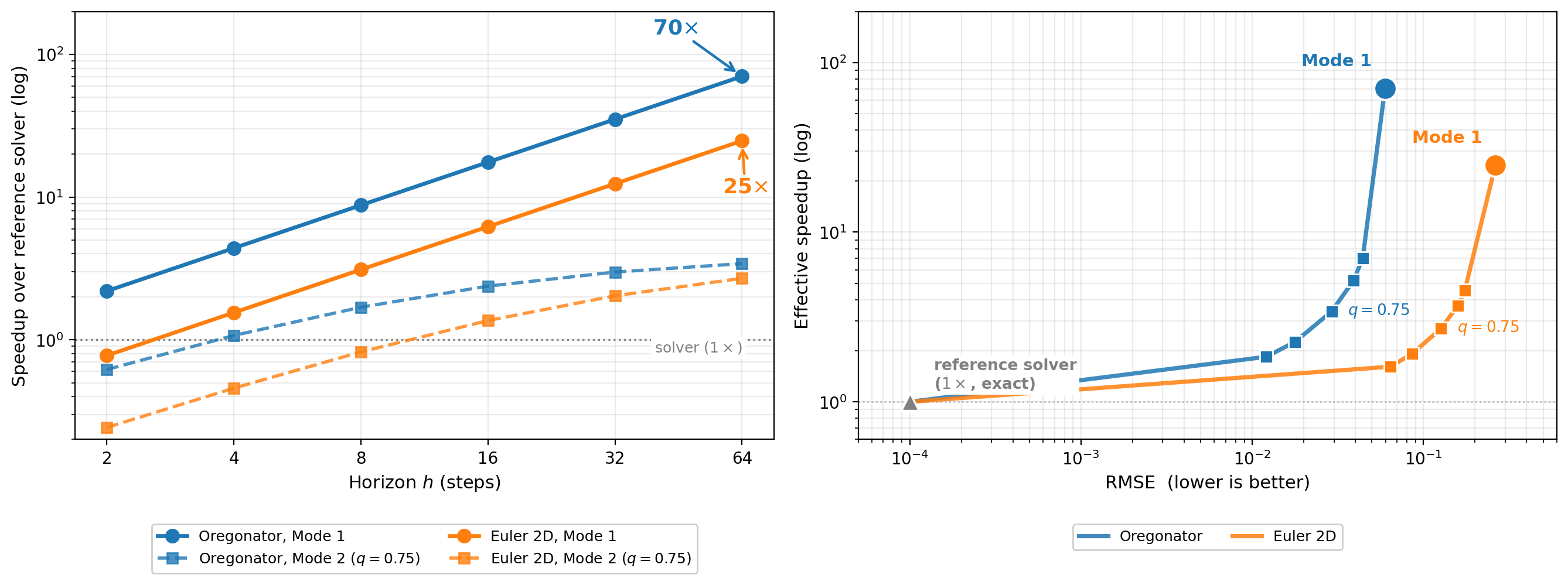
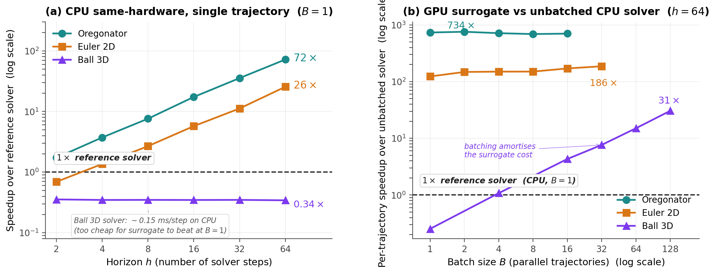
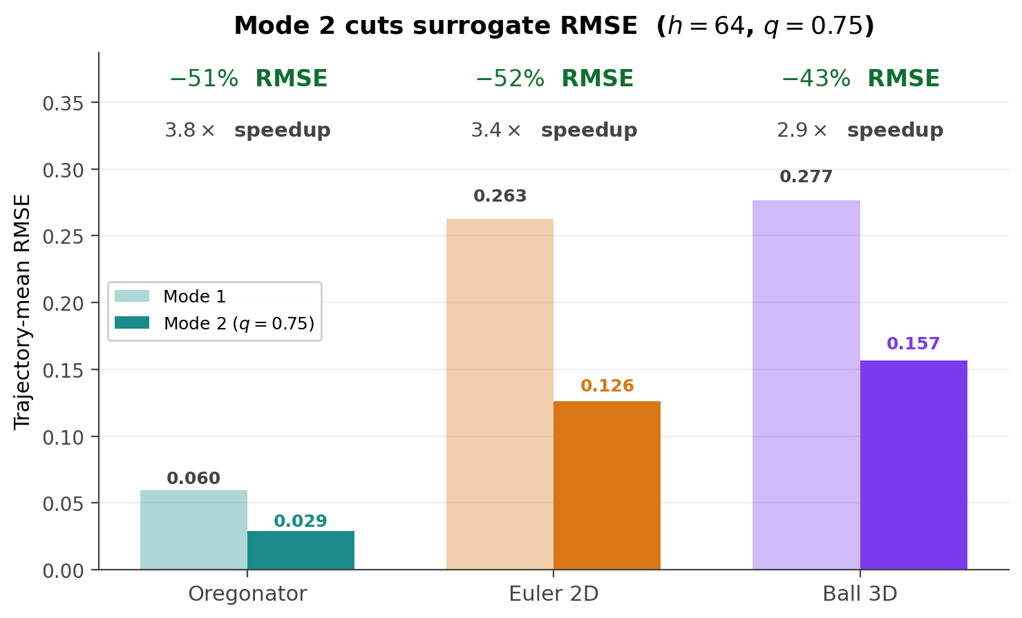
Abstract: Neural surrogates promise large speedups over classical solvers for physical dynamics but fail silently at sharp dynamical events such as shocks, fronts, and contact. We present hybrid neural world models for physical dynamics: a recipe for training and deploying multi-horizon surrogates in physical state space, where a single network with continuous horizon conditioning is trained with direct supervision against textbook reference solvers to predict any future state at horizon T in one forward pass. Although no part of the training data, loss function, or architecture supervises discontinuity location, the trained surrogate encodes it implicitly, recoverable from its forward passes alone as a per-trajectory error map that concentrates on shocks, fronts, and contacts, and stays small elsewhere. The map is competitive with or better than standard label-free baselines including deep ensembles, learned error heads, gradient-magnitude indicators, and locally-adaptive conformal prediction, while using only a single trained network and requiring no calibration set or governing-equation knowledge. The recipe supports two operating points. Mode 1 runs the surrogate alone for maximum throughput, with same-hardware CPU speedups of 26x to 72x against textbook solvers on the PDE environments. Mode 2 uses the error map to gate a reference-solver fallback, deferring uncertain trajectories and roughly halving the surrogate's residual error at the default operating point. The recipe applies without modification across reaction-diffusion, compressible Euler, and rigid-body collision dynamics.



Paper Prompts
Sign up for free to create and run prompts on this paper using GPT-5.
Top Community Prompts
Explain it Like I'm 14
Explaining “Hybrid Neural World Models” in Simple Terms
What this paper is about (overview)
This paper is about making fast, smart shortcuts for physics simulations using AI, and adding a built‑in “trust meter” so we can tell when the AI might be wrong. The goal is to get the speed of AI with the reliability of traditional (slower) physics solvers, especially around tricky events like shock waves, moving fronts, or bouncing collisions.
What the researchers wanted to find out (key questions)
The authors focused on three simple questions:
- Can one AI model quickly predict what a physical system will look like at any future time?
- Can we tell, without extra labels or physics code, when that AI’s prediction is likely untrustworthy?
- Can we combine the AI with a traditional solver in a smart way so we keep speed but avoid big mistakes?
How they did it (methods, with everyday analogies)
Think of a physics simulator like a careful, step‑by‑step recipe that’s slow but accurate. The authors train an AI “shortcut” that skips many steps to jump straight to a future state. Here’s the recipe they use:
- One model, many time horizons: The AI takes two inputs—what the system looks like now and “how far into the future” to look (call this T). It learns to predict the future in one go for many different T values. You can think of T as a knob that says “look 2 steps ahead” or “look 64 steps ahead.”
- Trained by a textbook solver: During training, the AI’s answers are checked against a trusted, classical simulator (the “textbook solver”). This teaches the AI to match the real physics.
- A simple trust test, no extra training: At test time, the AI is asked the same question two ways: 1) One long jump: “What happens after T?” 2) Two short jumps: “What happens after T/2, and then after another T/2?” If these two answers disagree a lot, that’s a warning sign. It’s like walking to a far point in one big stride versus two half‑strides—if you land in different places, your stride isn’t reliable on that terrain. The difference becomes an “error map” that highlights risky regions (for images) or a single risk score (for simple systems).
- Two modes of use:
- Mode 1: Use the AI alone for maximum speed.
- Mode 2: Use the AI’s trust score to decide. If it looks risky, send that case to the slow but accurate solver. If it looks safe, keep the AI’s answer. A single setting, called q, controls how cautious you are.
They tested this on three kinds of physics:
- Oregonator: chemical waves moving in a sheet (smooth fields with sharp moving fronts)
- Euler 2D: fast air/gas flows with shock waves (sharp jumps)
- Ball 3D: a ball bouncing in a box (sudden collision events)
What they found (main results and why they matter)
Here are the main takeaways:
- The AI is fast:
- On the two “fields” problems (chemical waves and fluid flow), using the AI alone was about 26× to 72× faster on the same CPU hardware than the traditional solver for long jumps into the future. On GPUs and in batches, the speedup can be much larger.
- The trust meter works:
- The “two short jumps vs one long jump” disagreement (the error map) reliably ranked which predictions were good and which were risky, across most tests. It highlighted exactly where sharp events happen (like fronts and shocks), which is where models often struggle.
- It outperformed or matched several common uncertainty tricks, like using multiple models (deep ensembles) or special learned “error heads,” while needing only one trained network and no extra calibration data.
- Smart fallback cuts errors a lot:
- In Mode 2, when the AI flagged the riskiest 25% of cases and sent those to the traditional solver, the overall prediction error dropped by roughly half, while still keeping about a 3× speedup. You can make it more cautious (more accurate, slower) or less cautious (faster, less accurate) by changing one knob (q).
- It works across different physics:
- The same method worked on chemical waves, fluid shocks, and bouncing balls without changing the core idea. That’s important because it suggests the trust meter is general, not a one‑off trick.
Why this is important (implications and impact)
- Faster science and engineering: Many fields—like weather forecasting, aerodynamics, and robotics—need lots of simulations. This approach can make them much faster while avoiding dangerous blind spots.
- Safer AI in physics: The built‑in trust signal means we can detect when the AI might be wrong, especially during sharp, surprising events. That’s crucial for real‑world use.
- Flexible, simple deployment: Only one model is needed. No extra “teacher” models, no special physics code during deployment, and no separate calibration process.
A few limits to keep in mind:
- The AI needs training data from a trusted solver for each new kind of system. It’s not zero‑shot magic.
- The trust signal can fail in rare, very unusual conditions (they found one such case for the bouncing ball with extreme settings).
- Speedups depend on how optimized your traditional solver is; if your solver is already heavily optimized on modern hardware, the gap shrinks.
Overall, this work shows a practical way to mix AI speed with solver reliability: run fast when it’s safe, and fall back to the exact method when it’s not. That balance could help many scientific and engineering tools run faster without sacrificing trust.
Knowledge Gaps
Knowledge gaps, limitations, and open questions
Below is a single, consolidated list of concrete gaps and open questions that remain unresolved and can guide future research:
- Calibrating the error map magnitude: how to convert the disagreement metric into calibrated absolute error estimates or risk bounds (e.g., expected RMSE), ideally without a large calibration set.
- Theoretical guarantees under non-smooth dynamics: formal conditions under which step-doubling reliably upper-bounds or correlates with true error near shocks/contacts, and characterization of counterexamples where “agreement but wrong” occurs (both one-shot and chained predictions are consistently wrong yet disagree little).
- Robust thresholding under strong covariate shift: methods to set and adapt the deferral threshold online when deployment distributions deviate strongly from validation, including drift detection and unsupervised calibration.
- Zero-/few-shot transfer across systems: whether a surrogate trained on one physical system (or range of parameters) can generalize to new PDEs/ODEs or parameter regimes without full re-training; what minimal data and adaptation are required.
- Continuous horizon conditioning fidelity: performance at arbitrary horizons not present in the training ladder and for non-dyadic splits (e.g., step-doubling when is unseen, or using chains), plus strategies to make the probe effective with non-geometric horizon sets.
- Adaptive horizon selection: using the error map to dynamically adjust per trajectory (or per region) to control accuracy and cost; policies and guarantees for horizon tuning at inference.
- Partial-domain solver handoff: algorithms and boundary-coupling schemes to defer only subregions of the spatial domain (AMR-like handoffs), including stencil compatibility and stability at surrogate–solver interfaces.
- Closed-loop rollout behavior: systematic evaluation of multi-step compounding error over long horizons (beyond one-pass to ), and whether the error map can trigger mid-horizon corrections or re-plans.
- Stochasticity and noise robustness: behavior of the probe under stochastic dynamics, measurement noise, and parameter uncertainty; methods to disentangle aleatoric from epistemic error in .
- Event-dominated failure regimes: alternative trust signals or hybrid schemes for contact-heavy or event-miscount failure modes (e.g., Ball 3D far-OOD restitution) where step-doubling underperforms.
- Real-time deployment constraints: analyzing worst-case latency and jitter when solver fallback is invoked, and designing schedules that meet real-time robotics constraints with bounded risk.
- Physics constraint compliance: quantifying and controlling conservation-law violations (mass, momentum, energy) by the surrogate; determining whether correlates with conservation errors and how to enforce constraints in training/inference.
- Data efficiency and training cost: estimating sample complexity and simulator time needed to reach target accuracy; cost–benefit models comparing training effort versus speedups at deployment.
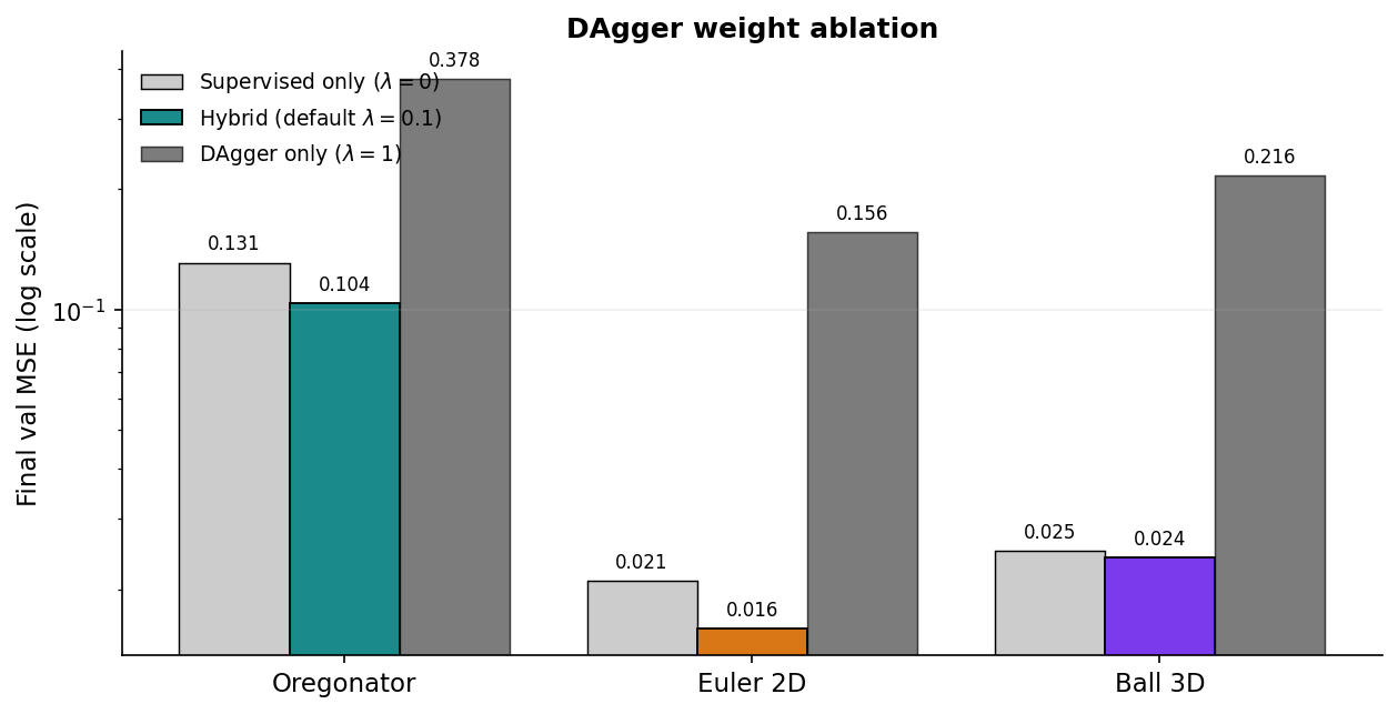
- Sensitivity to training recipe: rigorous ablations of FiLM conditioning, horizon set design, per-horizon loss weighting, and DAgger fraction (beyond 10%), with guidelines for stable and robust training.
- Scaling to 3D and larger grids: memory/computation trade-offs, speed/accuracy retention, and the effect on probe fidelity for 3D PDEs and high-resolution domains.
- Parameter variability in PDEs: training and evaluating across ranges of physical parameters (e.g., diffusion rate , gas constant ) to test robustness; meta-learning or conditional surrogates that generalize across parameter families.
- Combining trust signals: principled fusion of step-doubling with residual-based probes, deep ensembles, gradient indicators, or cycle-consistency to improve coverage when any single probe fails.
- Selective prediction guarantees: mapping the deferral fraction to target risk constraints (e.g., maximum RMSE or error quantiles), and deriving theoretical bounds for selective inference with .
- Detecting “agreement but wrong”: diagnostics to identify trajectories where one-shot and chained predictions agree but are both inaccurate (e.g., multi-split checks like chaining, diverse horizon ensembles).
- Complex contact dynamics: extension from a single ball with axis-aligned walls to multi-body frictional contact, oblique impacts, and compliant surfaces; assessing whether step-doubling remains informative.
- Fair speed comparisons: head-to-head evaluations versus optimized, vectorized solvers (JAX/CUDA, multi-GPU) and integrated pipelines, including the overhead of probe computation and fallback scheduling.
- Architectural diversity: testing the method across FNO, DeepONet, PINNs, and transformers to validate architecture-agnostic claims and identify inductive biases that affect probe quality.
- Metric choices and aggregation: impact of using physics-aware norms (e.g., weighted by conserved quantities) instead of per-channel , and robust aggregators (median/trimmed mean) for trajectory-level .
- Unsupervised threshold selection: developing label-free procedures (e.g., conformal or distribution-free methods) to set under covariate shift without relying on a representative validation set.
- Real-world datasets and sensing: evaluation on physical datasets with sensor noise, partial observability, and actuation uncertainty (e.g., robotics scene prediction), including deployment constraints and safety considerations.
- Formalizing smooth-region assumptions: methods to estimate Lipschitz constants and identify regions where the probe’s bound applies; validating these assumptions empirically per environment.
- Error-map operating characteristics: detailed false positive/negative analyses for deferral decisions, and procedures to tune the trade-off for application-specific costs of fallback vs. surrogate error.
- AMR integration protocols: concrete algorithms to guide refinement using , including refinement criteria, regridding, and consistency at surrogate–solver transitions.
- Memory/energy footprint: quantifying storage and energy savings versus ensembles or multi-network baselines, especially for edge deployment.
- Beyond- extrapolation: rigorous assessment of reliability when extrapolating to horizons longer than trained, and whether can predict when extrapolation becomes unsafe.
- Online refinement and active learning: using high- trajectories to incrementally retrain or fine-tune the surrogate (DAgger-style), with policies for sample selection and convergence guarantees.
Practical Applications
Overview
The paper introduces a practical recipe for fast, trust-aware neural surrogates for physical dynamics. A single multi-horizon model predicts future states at any horizon T in one pass and produces a label-free “error map” (via disagreement between T and two T/2 passes) that flags when and where it is unreliable. A two-mode deployment policy either runs the surrogate alone (Mode 1) for speed or defers selected trajectories to a reference solver (Mode 2) for accuracy. Validated on reaction–diffusion, compressible Euler with shocks, and rigid-body collisions, it yields 26×–72× CPU speedups on PDEs and halves residual error when using trust-aware fallback.
Below are concrete applications across sectors, grouped by deployment readiness. Each item notes likely tools/workflows and key assumptions or dependencies.
Immediate Applications
- CFD and CAE workflow acceleration with trust-aware fallback (sectors: aerospace, automotive, energy, manufacturing; software)
- What to do now: Integrate the surrogate and error map into design loops for aerodynamics, turbomachinery, wind/solar siting, and thermal management to pre-screen designs at high speed; route only high-risk cases (flagged by error map) to the CFD solver.
- Tools/workflows: Plugins for OpenFOAM/ANSYS/Star-CCM+; “Hybrid Surrogate Runner” that implements Mode 1/2 and a q-knob; dashboards that visualize per-cell error heatmaps for engineers.
- Assumptions/dependencies: Access to a reference solver for training and fallback; availability of a validation distribution to set the q-quantile threshold; training horizon ladder includes T and T/2; error map most reliable around shocks/fronts; solver–surrogate hardware parity for claimed speedups.
- Weather and environmental nowcasting triage (sectors: meteorology, hydrology, emergency management; public policy)
- What to do now: Use surrogate forecasts for rapid ensemble generation; defer to numerical weather prediction (NWP) in trajectories flagged by high error (e.g., near frontal passages or cyclogenesis). For flood and plume modeling, run surrogate for routine scenarios and trigger high-fidelity solvers for flagged cases.
- Tools/workflows: “Trust-aware forecast router” that runs Mode 2 over many initial conditions; integration with existing NWP and hydrological models; map overlays of error heatmaps for forecaster review.
- Assumptions/dependencies: Training on outputs from trusted NWP/physics models; validation data representative of deployment; semigroup-like behavior of dynamics over chosen horizons; provision for re-estimating thresholds under shift.
- Chemical/process engineering digital twins (sectors: chemicals, pharma, materials; operations)
- What to do now: Deploy reaction–diffusion surrogates to speed reactor monitoring and what-if analysis; use error maps to trigger high-fidelity solvers during transients (start-up/shutdown) when fronts emerge.
- Tools/workflows: Plant digital twin platforms with Mode 2 gating; online monitoring where high error prompts solver recalculation and potential control adjustments.
- Assumptions/dependencies: Accurate kinetics in training data; process-specific reference simulations for supervised training; manageable domain shifts during operation.
- Robotics simulation and planning with contact (sectors: robotics, logistics, manufacturing; software)
- What to do now: Accelerate physics for RL training or motion planning; use surrogate for free motion and defer near contacts flagged by the error score; in multi-agent scenes, triage trajectories with highest error to exact physics.
- Tools/workflows: Plugins for MuJoCo, Isaac Gym, PyBullet, Unity/Unreal; training loops that log the trajectory-level error scalar to schedule fallback or replanning.
- Assumptions/dependencies: Contact distributions at deployment similar to training; acknowledge degraded error ranking under extreme out-of-distribution restitution/gravity (as observed in the paper); maintain an exact physics engine in the loop for deferrals.
- Computer graphics and games physics acceleration (sectors: media, gaming)
- What to do now: Use surrogate for routine object dynamics; defer high-error trajectories (e.g., complex pile-ups) to the engine’s precise solver; use per-cell/trajectory error to drive level-of-detail or timestep adaptation.
- Tools/workflows: Middleware module for hybrid physics; runtime error heatmap visualizer for devs to tune q and timesteps.
- Assumptions/dependencies: Tolerance for small physical inaccuracies; engine support for selective handoff without noticeable latency spikes.
- Faster parameter sweeps and inverse problems in research (sectors: academia, R&D)
- What to do now: Run large sweeps with the surrogate; filter high-error trajectories for exact solver evaluation only; incorporate the error score as a label-free UQ signal in experiment design.
- Tools/workflows: HPC scripts that batch Mode 2 runs; scheduling based on the error quantile; reproducible pipelines with the provided horizon ladder.
- Assumptions/dependencies: Availability of training data from reference solvers; stable validation distribution to set thresholds; resource access for initial training.
- Adaptive mesh/timestep control using the error heatmap (sectors: scientific computing, software)
- What to do now: Use per-cell error maps to prioritize mesh refinement or smaller timesteps in solver runs, even if full per-region handoff isn’t implemented.
- Tools/workflows: AMR controllers that ingest surrogate error fields; mesh refinement policies that align to shock/contact localization.
- Assumptions/dependencies: Solver support for AMR; alignment between surrogate error hotspots and true truncation-error hotspots (empirically supported in paper).
- Label-free UQ baseline for physics surrogates (sectors: software, research)
- What to do now: Adopt step-doubling disagreement as a general-purpose, label-free trust signal for any trained multi-horizon surrogate where T and T/2 are available; replace deep ensembles or conformal UQ where calibration sets are impractical.
- Tools/workflows: UQ wrappers that compute T vs T/2 disagreement per trajectory/cell; dashboards ranking runs by risk.
- Assumptions/dependencies: Multi-horizon training including T/2; semigroup property approximately holds in the target dynamics; recognition that the score is directional (good at finding failures near non-smooth events).
- Education and outreach (sectors: education)
- What to do now: Interactive PDE/ODE sandboxes where students see predictions and corresponding error maps pinpointing fronts, shocks, and contacts in real time.
- Tools/workflows: Browser-based demos with sliders for horizon T and threshold q; overlays for error localization.
- Assumptions/dependencies: Pretrained surrogates on canonical PDEs included with the app.
Long-Term Applications
- Per-region hybrid solvers and domain-decomposed handoff (sectors: scientific computing, CAE)
- What it enables: Hand off only flagged subdomains to the reference solver while keeping the rest on the surrogate; couple across boundaries for stencil consistency.
- Tools/workflows: Solver modifications for partial-domain exchange, boundary synchronization, and AMR guided by error heatmaps.
- Assumptions/dependencies: Nontrivial engineering for boundary coupling; robust stability analysis for mixed domains; additional research to prevent artifacts at interfaces.
- Safety-critical autonomy with certifiable fallback (sectors: robotics, transportation)
- What it enables: Planning/control pipelines that run fast surrogates with a conservative deferral policy to exact physics, plus certification of worst-case risks.
- Tools/workflows: Runtime monitors using the error score; formal methods tying step-doubling signals to safety constraints; logging and auditing for regulators.
- Assumptions/dependencies: Stronger theoretical bounds under discontinuities; regulator-accepted validation; online recalibration under covariate shift.
- Cross-domain foundation surrogates for physics (sectors: software, cloud/AI platforms)
- What it enables: Pretrained multi-horizon surrogates covering families of PDEs/ODEs with plug-and-play error maps; fine-tuned per system.
- Tools/workflows: Model hubs exposing inference APIs that return both predictions and error maps; auto-tuning of q based on user-supplied validation slices.
- Assumptions/dependencies: Large-scale curated simulator datasets; compute for pretraining; domain-adaptation strategies when semigroup or state normalization differs.
- Real-time, city-scale digital twins (sectors: smart cities, energy, HVAC, urban planning)
- What it enables: Continuous fluid/thermal simulations for buildings, microclimate, pollution dispersion with fast surrogates and solver deferrals during events (e.g., heatwaves, inversions).
- Tools/workflows: Streaming data assimilation; dynamic q scheduling under changing conditions; per-region AMR and solver handoff when local error spikes.
- Assumptions/dependencies: Sensor networks for calibration; robust online thresholding under nonstationary shifts; scalable solver-in-the-loop infrastructure.
- Patient-specific cardiac and bioelectric simulations (sectors: healthcare, medical devices)
- What it enables: Rapid what-if analyses of arrhythmias, ablation planning, or drug effects; fallback to high-fidelity solvers during wavefront interactions.
- Tools/workflows: Clinical planning software integrating reaction–diffusion surrogates; visualization of error maps to highlight uncertain regions for clinicians.
- Assumptions/dependencies: Access to patient-specific models and ground-truth simulators; regulatory validation; careful handling of OOD physiology and safety.
- Subsurface and geothermal reservoir management (sectors: energy, geoscience)
- What it enables: Fast scenario evaluation for injection/production planning; error-triggered high-fidelity runs near fronts (e.g., waterflood fronts or CO₂ plume edges).
- Tools/workflows: Integration with reservoir simulators (e.g., Eclipse, TOUGH, Open Porous Media); hybrid scheduling across ensembles.
- Assumptions/dependencies: Extension to porous media PDEs and multi-phase flow; availability of training data; verification that error maps localize fronts in these systems.
- Climate and insurance risk analytics (sectors: insurance, finance, public sector)
- What it enables: Larger ensembles for peril modeling (wind, surge, flood) with trust-aware routing of extreme-event trajectories to full simulators; improved turnaround for pricing and policy stress tests.
- Tools/workflows: Pipelines that tag high-uncertainty members using the error score; reporting that separates surrogate-credible vs deferred runs.
- Assumptions/dependencies: Representative training and validation distributions; governance around model risk and uncertainty reporting.
- Online active learning and continual improvement (sectors: software, MLOps)
- What it enables: Use deferred trajectories as high-value data for periodic retraining (DAgger-like loops), reducing future deferrals and improving accuracy where it matters.
- Tools/workflows: Data stores capturing solver fallbacks; scheduled retraining with horizon ladders; monitoring of AUROC and error–defer curves over time.
- Assumptions/dependencies: Stable data pipelines; safeguards against catastrophic forgetting; compute budgets for regular retraining.
- Standards and policy for hybrid AI–physics systems (sectors: policy, standards bodies)
- What it enables: Best-practice guidelines for deploying surrogates with label-free trust signals, including thresholding, monitoring, and reporting.
- Tools/workflows: Compliance checklists; benchmark suites that include trust-aware metrics (AUROC, defer curves) beyond RMSE.
- Assumptions/dependencies: Community consensus on evaluation under shift; cross-sector case studies to inform thresholds and governance.
Common Assumptions and Dependencies Across Applications
- A reference solver is available to generate training pairs and to serve as the fallback in Mode 2.
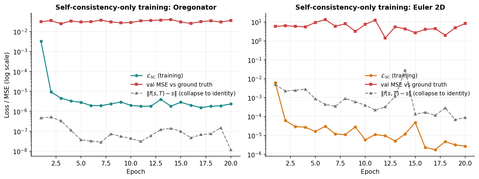
- Multi-horizon training includes both T and T/2 (laddered horizons) and direct supervision against solver outputs; self-consistency alone is insufficient.
- The error map is especially reliable around non-smooth features (shocks, fronts, contacts); it may degrade under extreme OOD conditions unrelated to step-size sensitivity.
- Thresholds for deferral are set on a validation set representative of deployment; stronger distribution shifts require re-estimation or online adaptation.
- Partial-domain handoff and AMR require solver support and careful boundary coupling (future work).
- Speedups depend on hardware and solver vectorization; same-hardware CPU comparisons in the paper provide conservative baselines.
Glossary
- AdamW: An optimization algorithm that decouples weight decay from the gradient update in Adam. "All three surrogates are trained with the same recipe: AdamW, multi-horizon supervision over , and a DAgger \citep{ross2011dagger} refinement against the reference solver."
- AdaLN: Adaptive Layer Normalization, a conditioning mechanism for neural networks. "we use FiLM rather than AdaLN, concatenation, or cross-attention because it is parameter-light and slots cleanly into both architectures without redesign."
- Amortised multi-step prediction: Learning to approximate multiple simulation sub-steps in a single forward pass. "A separate thread amortises multiple sub-steps into a single forward pass."
- AUROC: Area Under the Receiver Operating Characteristic curve; a scalar that measures ranking quality. "Table~\ref{tab:auroc_sd_coverage} reports step-doubling AUROC against true error across all $54$ cells (three environments, six training horizons, three distribution splits)."
- Belousov–Zhabotinsky reaction: A classic oscillating chemical reaction modeled by the Oregonator system. "The Oregonator \citep{field1972oregonator,tyson1980oregonator} is a two-variable reaction-diffusion model of the Belousov--Zhabotinsky oscillating chemical reaction;"
- CFL condition: Courant–Friedrichs–Lewy stability condition controlling time step size in explicit solvers. "Euler 2D: finite-volume HLL Riemann solver \citep{harten1983hll} with and ."
- Conformal prediction: A framework for distribution-free predictive intervals calibrated on held-out data. "Conformal prediction \citep{romano2019conformalized,bostroem2017accelerating,tibshirani2019conformal,angelopoulos2023conformal} gives distribution-free intervals but needs a calibration set and degrades under shift."
- Contact discontinuity: A surface across which fluid properties change abruptly without a shock in pressure. "The dynamics produce shocks, contact discontinuities, and smooth rarefactions, often interacting."
- Conserved-variable field: A representation of fluid state in terms of conserved quantities like mass, momentum, and energy. "The state is a four-channel conserved-variable field on a grid, satisfying"
- Covariate shift: A change in the input distribution between training and deployment. "under stronger covariate shift than our OOD-far split, may need re-estimation online."
- DAgger: Dataset Aggregation; an imitation-learning algorithm that iteratively queries an expert to refine training data. "All three surrogates are trained with the same recipe: AdamW, multi-horizon supervision over , and a DAgger \citep{ross2011dagger} refinement against the reference solver."
- Deep ensembles: A predictive uncertainty method that averages predictions from multiple independently trained networks. "Deep ensembles \citep{lakshminarayanan2017simple,ovadia2019can} remain the standard label-free UQ baseline but cost to train and store; we match a ensemble at one-third the cost."
- FiLM: Feature-wise Linear Modulation; a lightweight conditioning layer for neural networks. "The horizon is encoded as a continuous embedding via FiLM \citep{perez2018film};"
- Finite-volume method: A discretization technique that enforces conservation laws by integrating fluxes over control volumes. "Euler 2D: finite-volume HLL Riemann solver \citep{harten1983hll} with and ."
- Flow map: The operator that advances a dynamical system’s state forward in time by a given horizon. "Let be the physical state at time and the ground-truth flow map that advances the state by horizon ."
- Fourier neural operator: A neural architecture that learns operators (e.g., PDE solution maps) using spectral convolutions. "Fourier neural operators \citep{li2021fno}, DeepONet \citep{lu2021deeponet}, and physics-informed networks \citep{raissi2019pinns} are the architectural primitives that motivated neural-replacement solvers;"
- FTCS: Forward Time Centered Space; an explicit finite-difference scheme for diffusion and similar PDEs. "implicit Euler for the stiff reaction term, explicit FTCS for diffusion with internal CFL substepping;"
- HLL Riemann solver: A Godunov-type approximate Riemann solver (Harten–Lax–van Leer) for hyperbolic conservation laws. "Euler 2D: finite-volume HLL Riemann solver \citep{harten1983hll} with and ."
- Ideal-gas closure: The relation that closes Euler equations by linking pressure and energy via the ideal gas law. "with the standard ideal-gas closure relating energy to pressure."
- Inviscid: Describing flow with negligible viscosity. "The 2D compressible Euler equations govern inviscid mass--momentum--energy conservation in supersonic aerodynamics, blast waves, and astrophysical jets."
- Lipschitz (L-Lipschitz): A regularity condition bounding how much a function can change relative to input changes. "On a region where the per-horizon error is uniformly bounded by , is -Lipschitz, and chained predictions stay in ,"
- Multi-horizon surrogate: A single model conditioned on prediction horizon to forecast multiple future times. "We train a multi-horizon surrogate: a network with continuous horizon conditioning that predicts any future state at horizon in one forward pass."
- Pareto frontier: The set of trade-off optimal points balancing competing metrics (e.g., error vs speed). "Pareto frontier in (RMSE, speedup) space at ."
- Reaction–diffusion PDE: A partial differential equation combining local reactions with spatial diffusion. "Oregonator (a reaction-diffusion PDE with propagating chemical fronts)"
- Rarefaction: A smooth expansion wave in compressible flow where characteristics diverge. "The dynamics produce shocks, contact discontinuities, and smooth rarefactions, often interacting."
- Restitution: The coefficient determining the elasticity of collisions (ratio of post- to pre-impact normal velocity). "restitution "
- Richardson extrapolation: A technique that estimates and reduces discretization error by comparing solutions at multiple step sizes. "Classical Richardson extrapolation \citep{dormand1980family,richardson1911} compares two solver legs of known order of convergence;"
- Rigid-body ODE: An ordinary differential equation governing the motion of a solid object without deformation. "Ball 3D (a rigid-body ODE with collision events)."
- Runge–Kutta (embedded): A family of ODE solvers; embedded variants provide error estimates from paired formulas. "Embedded Runge-Kutta methods \citep{dormand1980family} and Richardson extrapolation \citep{richardson1911} estimate local truncation error by comparing two solver legs of \emph{known order of convergence}."
- Schulz–Rinne configuration: A benchmark initial condition for 2D Euler equations exhibiting interacting waves. " concentrates ... on the four contact discontinuities of the Schulz--Rinne configuration in Euler,"
- Self-consistency loss: A training objective enforcing consistency across steps/horizons, which here collapses to identity mapping without supervision. "Appendix~\ref{app:self_consistency} shows the self-consistency loss of \citet{frans2024shortcut}, when ported from diffusion to physical state, collapses to the identity map;"
- Semigroup composition property: The property that time evolution composes additively, i.e., evolving by equals evolving by then by . "The true flow satisfies the semigroup composition property "
- Shock (in PDEs): A discontinuity in fluid variables (e.g., density, pressure) arising in hyperbolic conservation laws. "Neural surrogates promise large speedups over classical solvers for physical dynamics but fail silently at sharp dynamical events such as shocks, fronts, and contact."
- Semi-implicit Euler: A time-stepping method that treats some terms implicitly and others explicitly for stability. "pure-NumPy rigid-body integrator with semi-implicit Euler at $50$ substeps per saved frame and analytic axis-aligned wall collisions;"
- Step-doubling: Comparing a single-step prediction at horizon with two chained half-steps at to gauge error. "Table~\ref{tab:auroc_sd_coverage} reports step-doubling AUROC against true error across all $54$ cells"
- Strang splitting: A second-order operator-splitting technique alternating sub-steps for different parts of a PDE. "Oregonator: Strang-split integrator on a periodic grid;"
- Tyson reduction: A reduced-form kinetic model for the Oregonator reaction dynamics. "with the diffusion rate and the Tyson reduction of the reaction kinetics."
- U-Net: A convolutional encoder–decoder architecture with skip connections, popular for dense prediction on grids. "a U-Net \citep{ronneberger2015unet} for two-dimensional grid-structured PDE fields, where its multiscale receptive field matches the spatial structure of fronts and shocks,"
- Uncertainty quantification (UQ): Techniques that estimate predictive uncertainty or confidence in model outputs. "Deep ensembles \citep{lakshminarayanan2017simple,ovadia2019can} remain the standard label-free UQ baseline but cost to train and store;"
Collections
Sign up for free to add this paper to one or more collections.