Beyond Independence: on Jointly Normal Priors in Bayesian Inversion

Abstract: We consider joint inversion for two or more unknown parameters from observational data in the Bayesian framework. Standard approaches often either treat the parameters as independent or impose structural similarity through regularisation terms that can be difficult to interpret statistically. We instead construct jointly Gaussian prior models with prescribed Gaussian marginals, so that correlation between the parameters can be incorporated without altering the marginal prior distributions. We propose a joint covariance construction that preserves the marginals, allows spatially varying cross-correlation, and supports uncertainty and inference in the correlation itself. The construction is valid for any strict contraction encoding the desired cross-correlation and is optimal in a canonical correlation sense under the principal square root factorisation. We demonstrate the method using prior sampling and several inference examples: a low-dimensional illustrative example and two higher-dimensional examples, including a PDE-constrained problem. The examples highlight both the potential pitfalls of ignoring or neglecting uncertainty in the correlation as well as reinforcing a key principle of the Bayesian paradigm: unknown quantities included in a model should be treated as random variables.

• The paper introduces a novel joint Gaussian prior construction that preserves individual marginals while enabling spatially varying cross-correlation inference.
• It employs principal square root factorisation to optimize the canonical correlation structure and supports efficient sampling via adaptive MCMC and dimension reduction.
• Hierarchical inference over the cross-correlation parameter improves uncertainty quantification and yields robust parameter estimation in multi-parameter models.

Jointly Normal Priors for Bayesian Inversion: Construction, Inference, and Uncertainty Quantification

Introduction and Motivation

The paper "Beyond Independence: on Jointly Normal Priors in Bayesian Inversion" (2605.00332) addresses a critical limitation in the prevalent practice of Bayesian inversion for multi-parameter models: the assumption of prior independence between parameter fields. While independent priors are computationally convenient, they fail to represent structural or physical relationships between parameters and cannot propagate or quantify uncertainty in the correlation between unknowns. This work introduces a principled construction of jointly Gaussian priors, preserving the prescribed marginals of individual parameters, but enabling explicit encoding—and inference—of spatially varying cross-correlation.

The main contribution is a family of joint covariance structures for high-dimensional parameters that explicitly preserve marginal distributions, flexibly encode prescribed correlation or contraction operators, and support efficient sampling and inference for the correlation (or hyper-) parameters themselves. The construction admits both constant and spatially heterogeneous correlation and is optimal in the canonical correlation sense when principal square root factorisation is adopted.

Construction of Joint Gaussian Priors

The methodology constructs a joint Gaussian prior for parameters $p \in \mathbb{R}^{n_1}$ and $m \in \mathbb{R}^{n_2}$, given marginal Gaussians $\mathcal{N}(p_\ast, \Gamma_p)$ and $\mathcal{N}(m_\ast, \Gamma_m)$. The joint prior $\mathcal{N}((p_\ast, m_\ast), \Gamma)$ has a block structure:

$$\Gamma = \begin{pmatrix} \Gamma_p & L_p^{-1} C L_m^{-T} \ L_m^{-1} C^T L_p^{-T} & \Gamma_m \end{pmatrix}$$

where $L_p$, $L_m$ are chosen factorizations of the marginals' precision matrices and $C$ is a user-prescribed contraction encoding desired cross-correlation. For $C$ a strict contraction, this yields a valid covariance with correct marginals. Notably, with principal square roots, the construction matches $m \in \mathbb{R}^{n_2}$0 in canonical correlation space, giving a unique optimal solution for matching the desired cross-correlation structure.

Efficient sampling from the joint is facilitated by explicit whitening and defect operators; analytical forms for both full and conditional sampling and their factor properties are given, ensuring no significant computational penalty relative to independent priors for sampling.

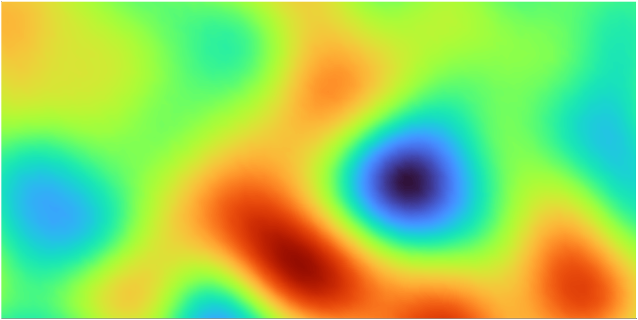
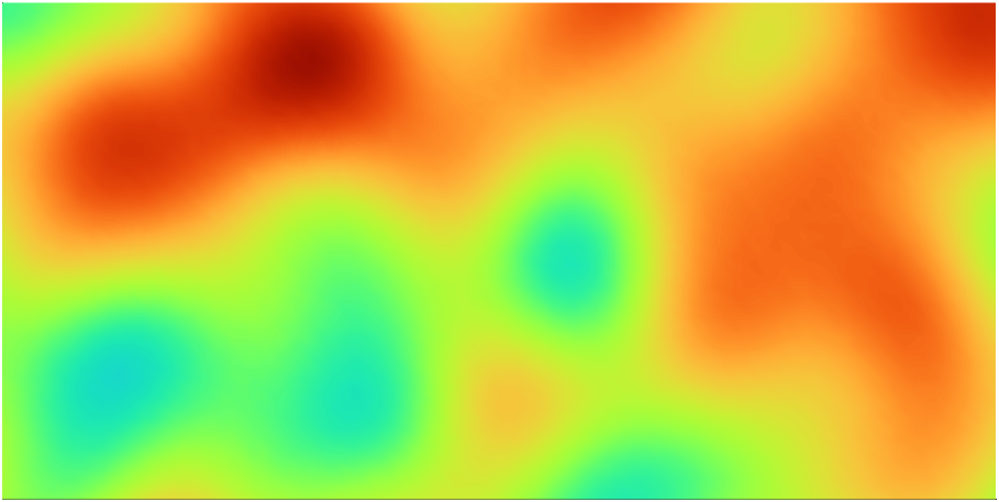
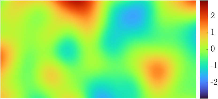
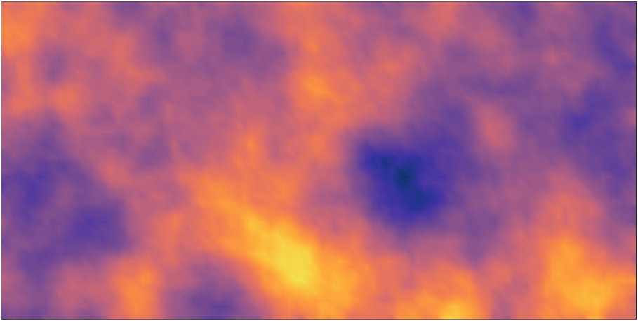
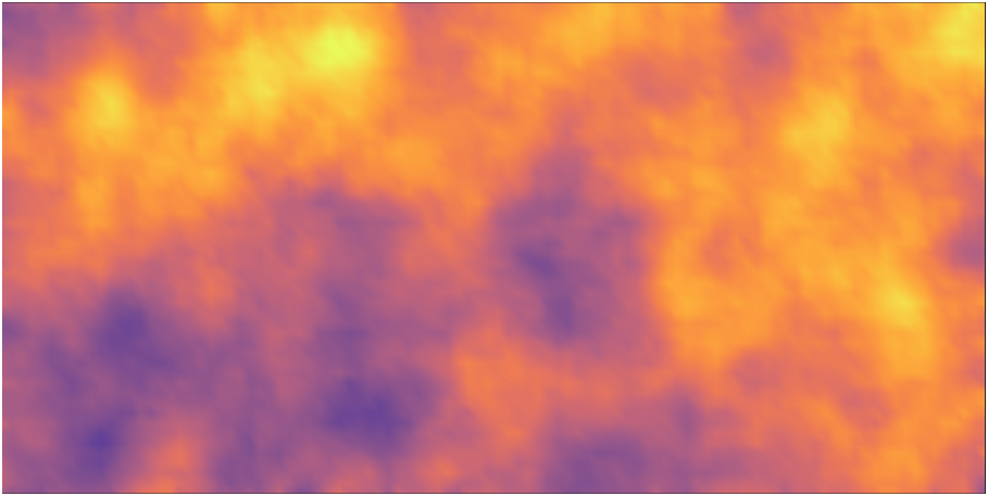
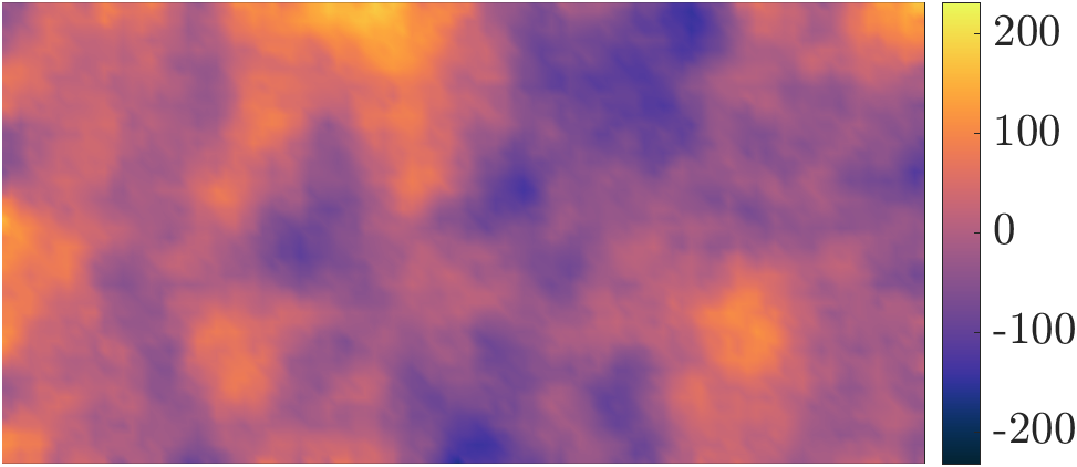
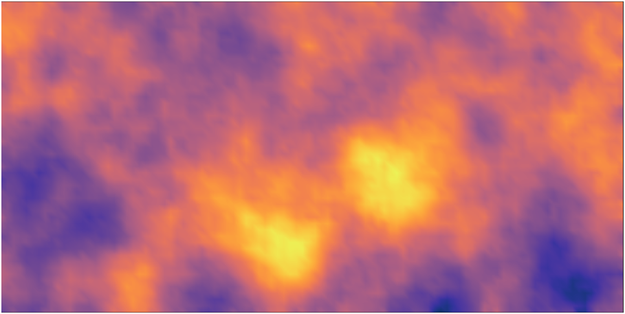
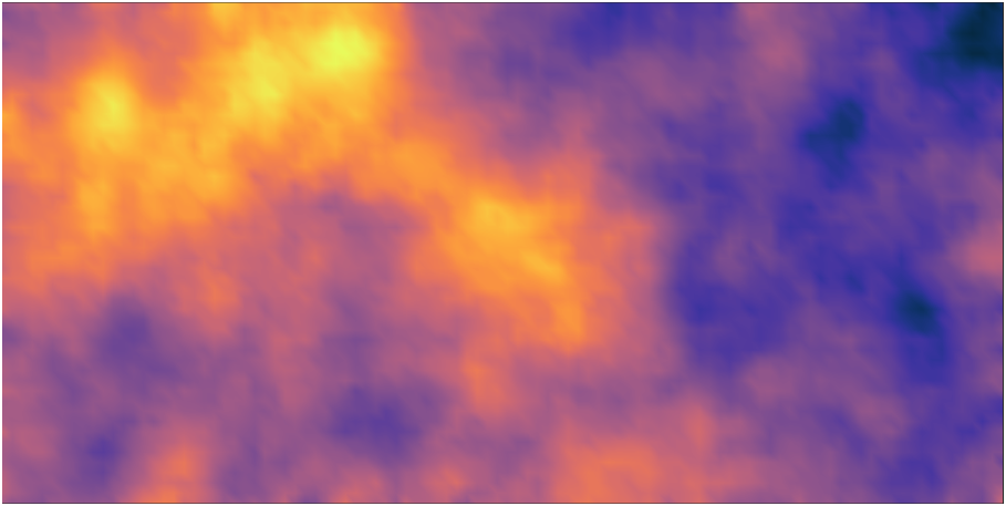
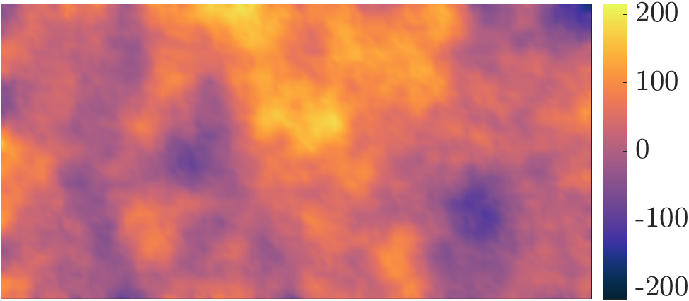
Figure 1: Samples from the joint prior in Example 1, demonstrating flexible, spatially heterogeneous correlation structures generated by the proposed construction.

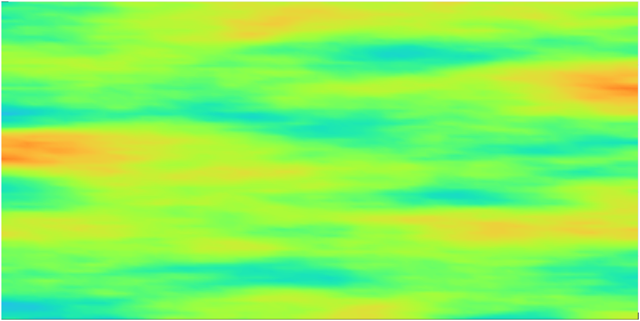
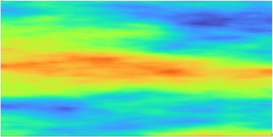
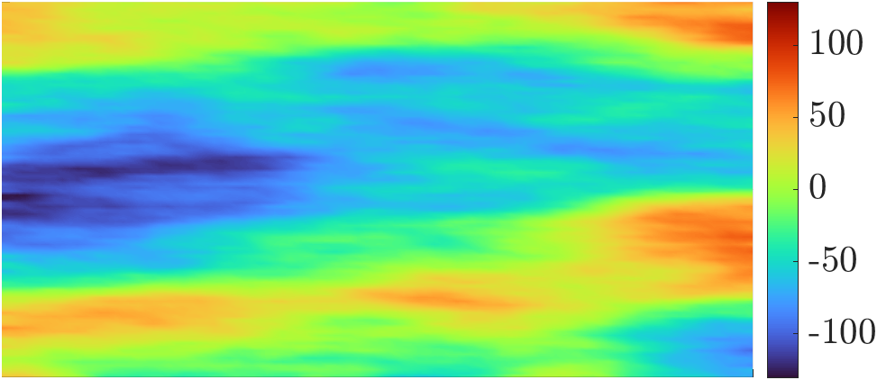
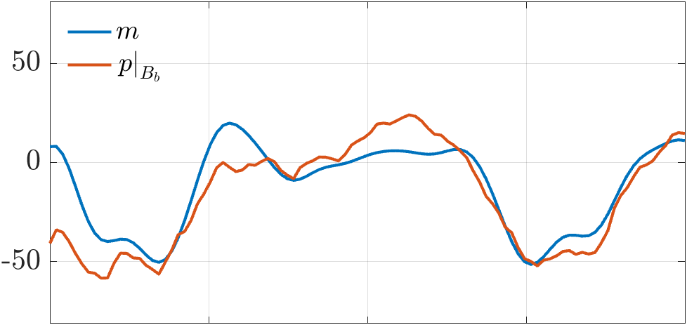
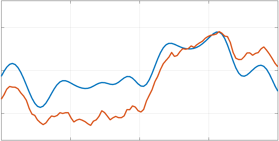
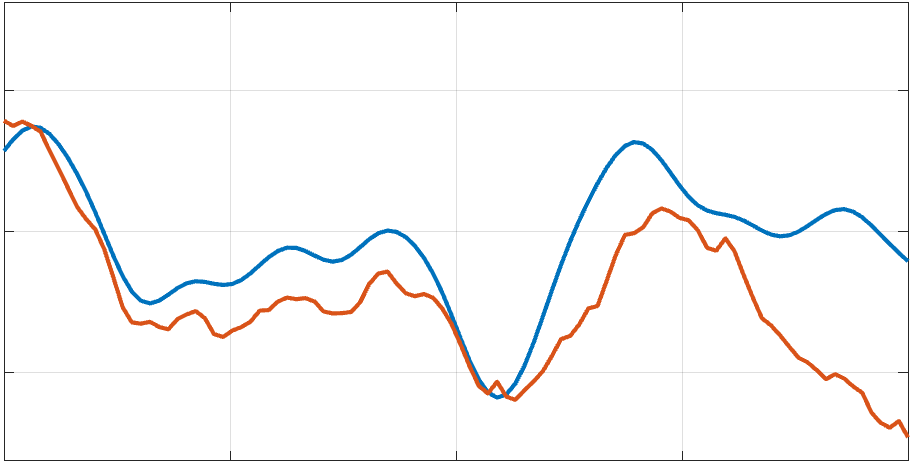
Figure 2: Samples from the joint prior for parameters of different dimensions and support—demonstrating the extension to 2D-1D coupling with spatially localized cross-correlation.

Factorisation and Encoding of Cross-Correlation

The choice of factorisation for the prior precision/square-root (principal square root vs. Cholesky) materially alters the induced cross-correlation structure. The principal square root factorisation preserves symmetry and spatial locality, whereas the Cholesky factorisation induces unwanted triangular/casual cross-correlations due to its non-symmetric nature—potentially leading to artefactual parameter relationships.

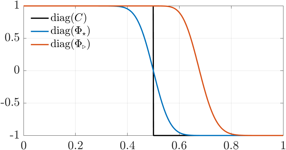
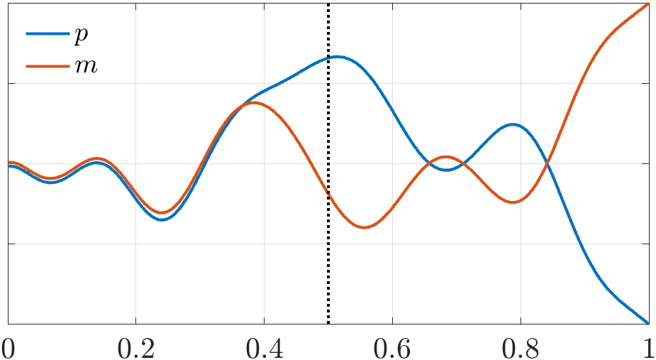
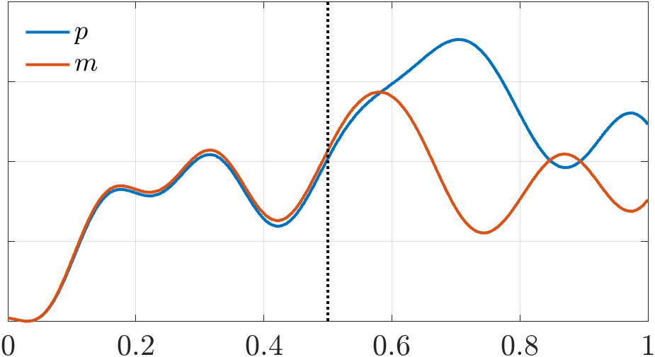
Figure 3: Comparison of cross-correlation realised using principal square root (correct) and Cholesky factor (skewed) factorizations for the joint prior, highlighting the critical role of operator choice.

Uncertainty in Cross-Correlation: Hierarchical Inference

The framework enables full Bayesian treatment of the correlation structure itself. Rather than assuming a fixed $m \in \mathbb{R}^{n_2}$1, the paper advocates placing a hyperprior (e.g., a uniform over the space of contractions or a more structured parametric family) on $m \in \mathbb{R}^{n_2}$2, making it a random variable inferred jointly with $m \in \mathbb{R}^{n_2}$3 and $m \in \mathbb{R}^{n_2}$4. The resulting hierarchical model:

$m \in \mathbb{R}^{n_2}$5

allows the posterior to propagate data-driven uncertainty in both parameter fields and their cross-correlation, in direct contrast to the overconfident or over-constrained inferences of standard approaches.

Inference Algorithms and Dimension Reduction

The resulting posteriors, particularly when $m \in \mathbb{R}^{n_2}$6 is endowed with a prior, are generally non-Gaussian and can only be characterised accurately via sampling-based methods. An adaptive Metropolis-within-Gibbs (MwG) MCMC sampler is developed which alternately samples the primary parameters conditional on $m \in \mathbb{R}^{n_2}$7, and $m \in \mathbb{R}^{n_2}$8 conditional on the parameter fields. For high-dimensional fields (e.g., FEM or Gaussian process priors), the approach leverages truncated Karhunen-Loève expansions for aggressive dimension reduction without meaningful loss of information.

Numerical Experiments

Low-Dimensional Example: Monod Model

A toy example using the Monod bacterial growth model explores the sensitivity of inference to the assumed cross-correlation. The work demonstrates that credible regions and posterior support for the true parameter values are strongly affected by the prior correlation $m \in \mathbb{R}^{n_2}$9; mis-specification yields biased and poorly calibrated posteriors with false overconfidence. Treating $\mathcal{N}(p_\ast, \Gamma_p)$0 as unknown and inferring it along with the physical parameters yields superior credible coverage and robust uncertainty quantification.

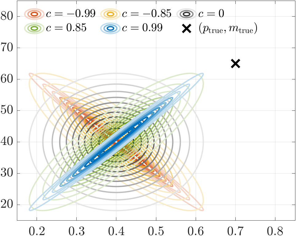
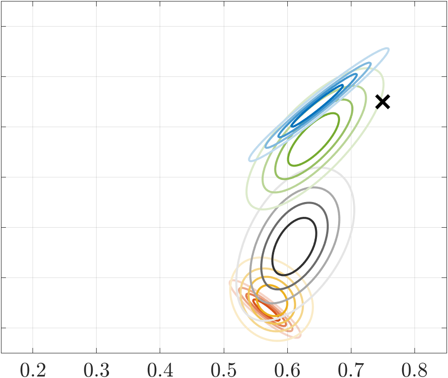
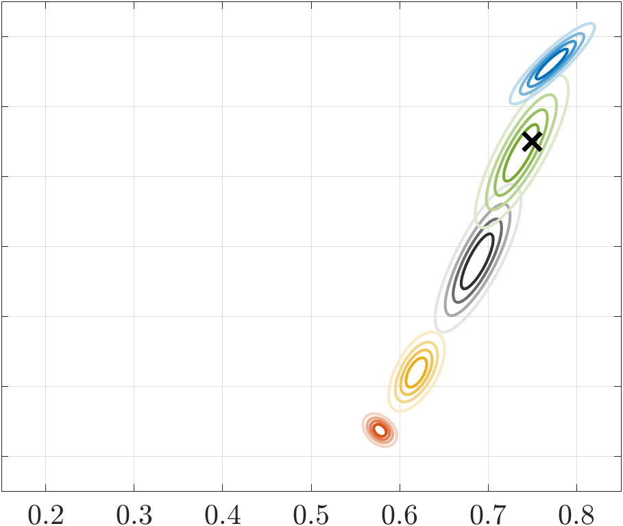
Figure 4: Joint prior and posterior distributions for the Monod model, illustrating the sensitivity of inference to correlation specification and the improvement from inferring $\mathcal{N}(p_\ast, \Gamma_p)$1 as an unknown.

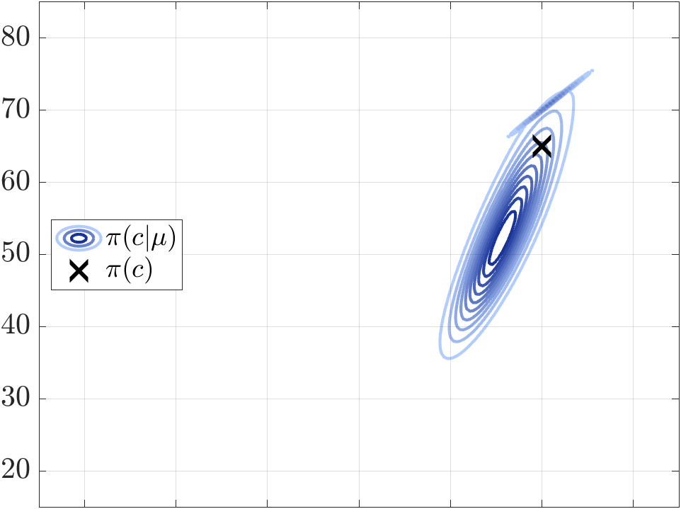
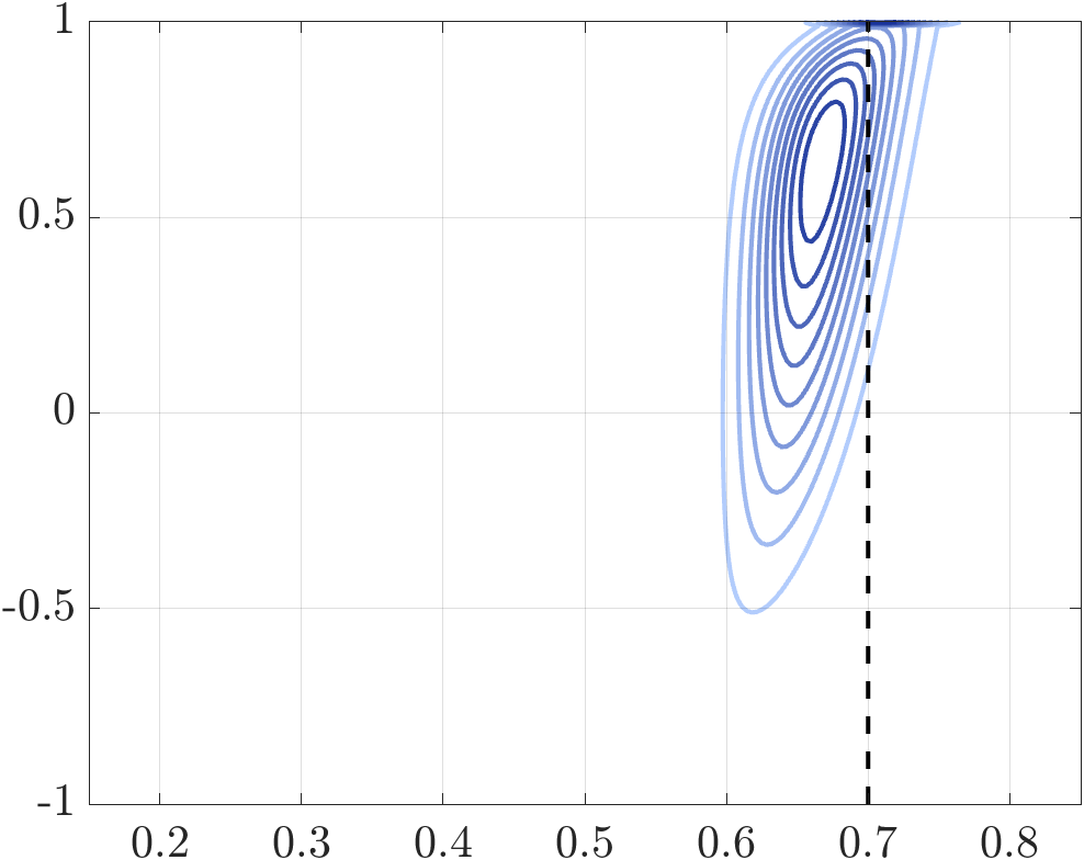
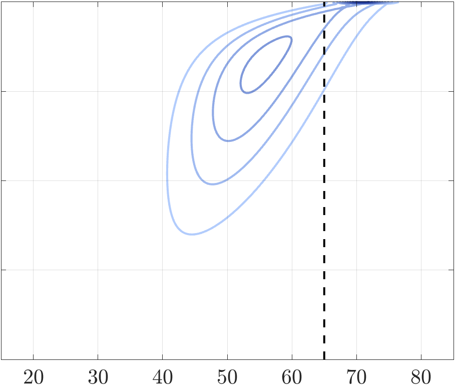
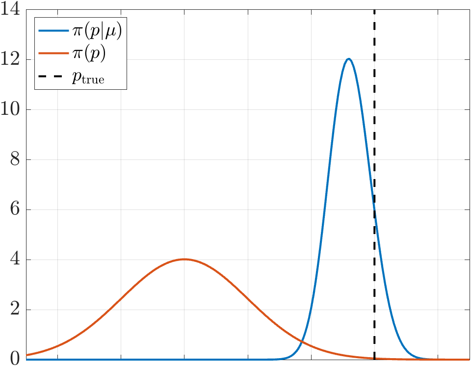
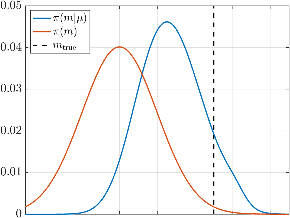
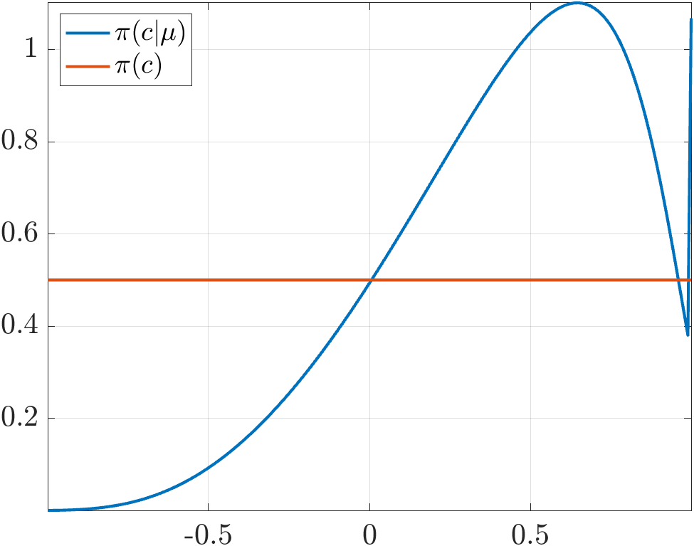
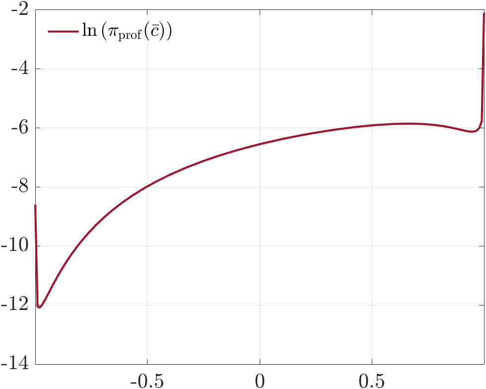
Figure 5: Corner plot for the posteriors of $\mathcal{N}(p_\ast, \Gamma_p)$2 in the Monod model with $\mathcal{N}(p_\ast, \Gamma_p)$3 random: robust uncertainty quantification and correct support for the physical truth.

High-Dimensional Examples: Co-Kriging and Subsurface Flow

Example 1: Co-Kriging

Spatial fields $\mathcal{N}(p_\ast, \Gamma_p)$4 and $\mathcal{N}(p_\ast, \Gamma_p)$5 are estimated jointly from spatially disjoint observations. Independent inference confines posterior concentration to local measurement regions. The proposed joint inference with correlation estimation propagates information globally, yielding lower posterior variance and improved reconstruction for both fields, as measured by error metrics and effective sample size.

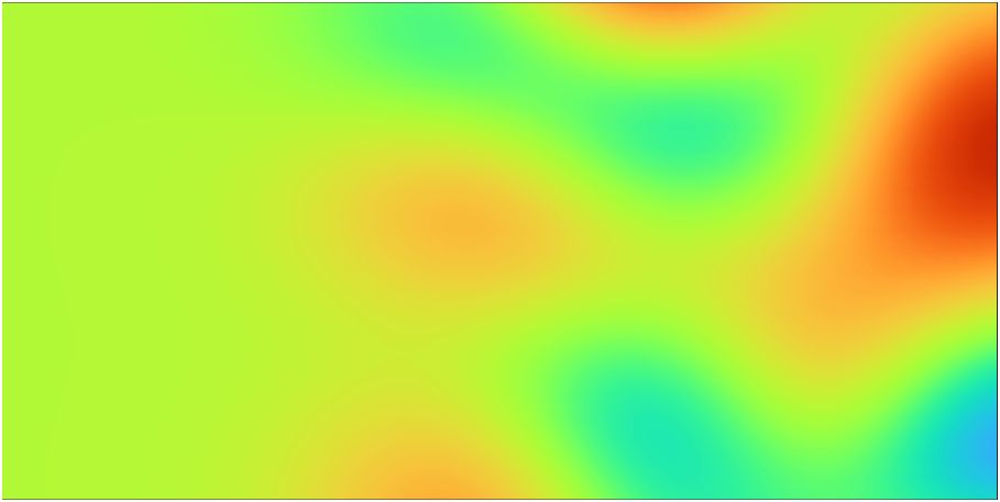
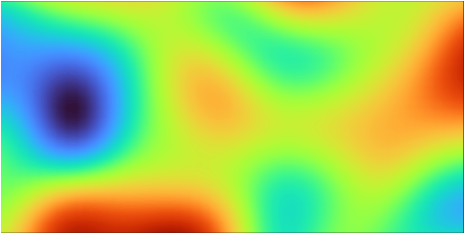
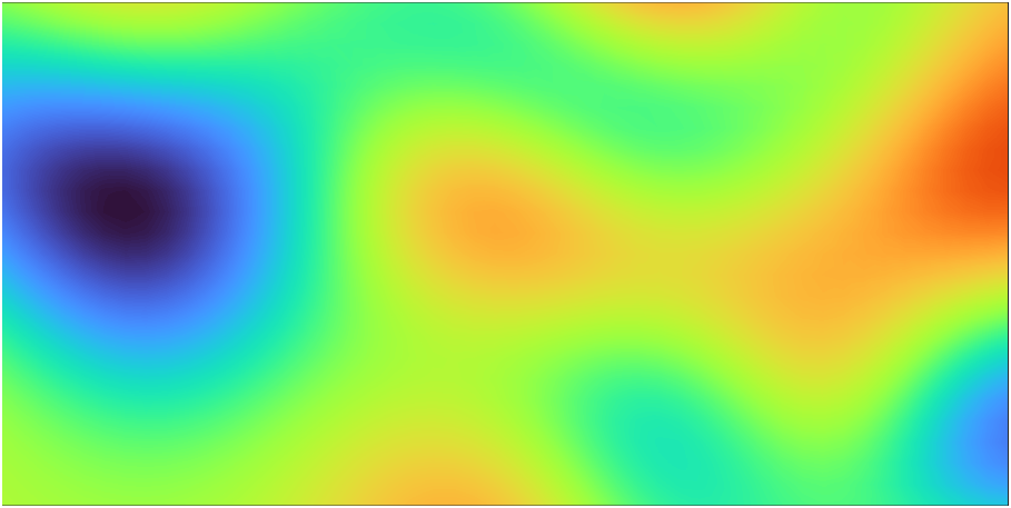
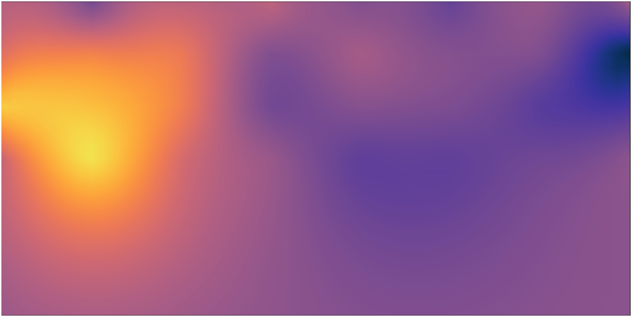
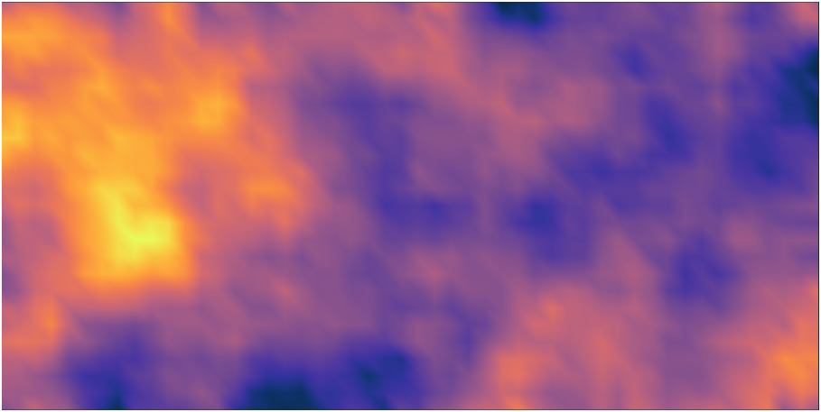
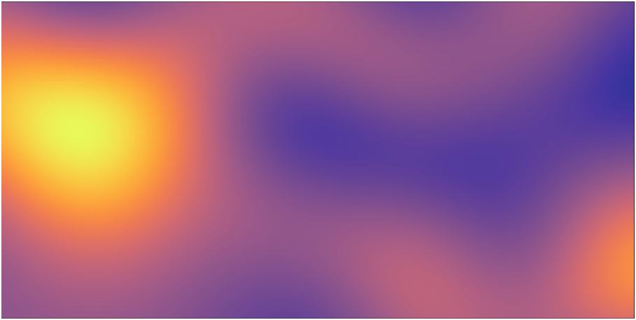
Figure 6: True fields and conditional mean estimates in the co-kriging example—joint inference yields clear improvements over independent inversion.

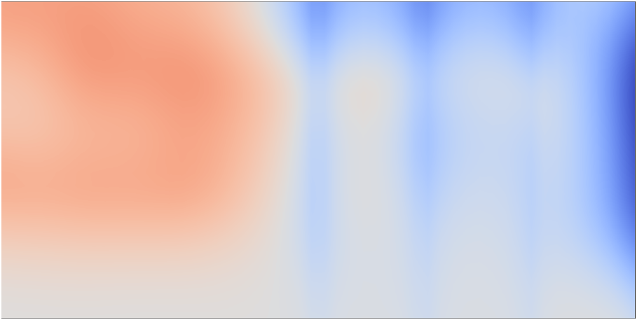
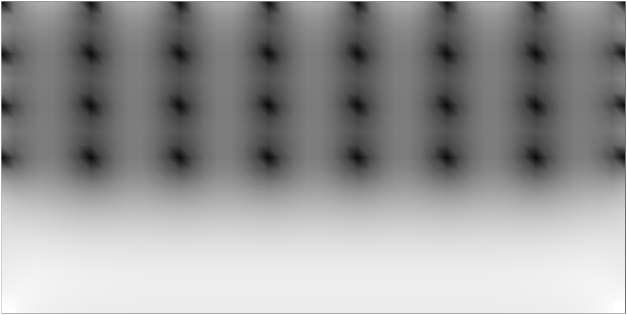
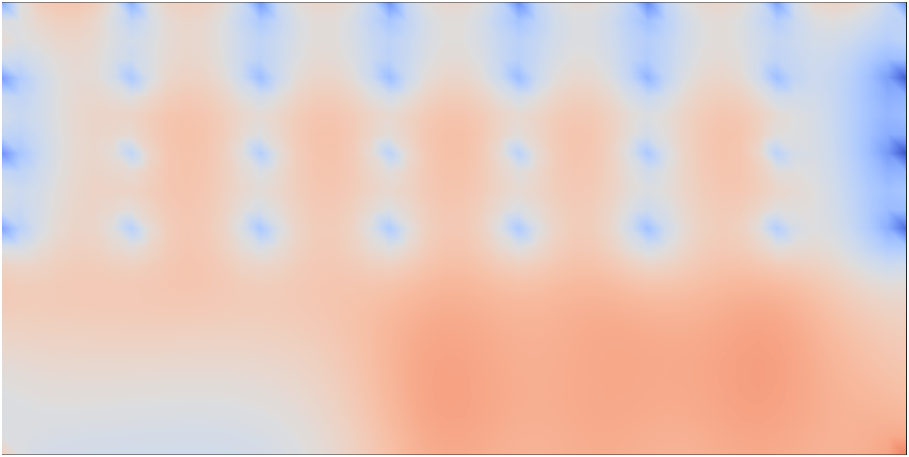
Figure 7: Pointwise reduction in posterior standard deviation for $\mathcal{N}(p_\ast, \Gamma_p)$6 and $\mathcal{N}(p_\ast, \Gamma_p)$7, showing enhanced information transfer between fields under joint inference.

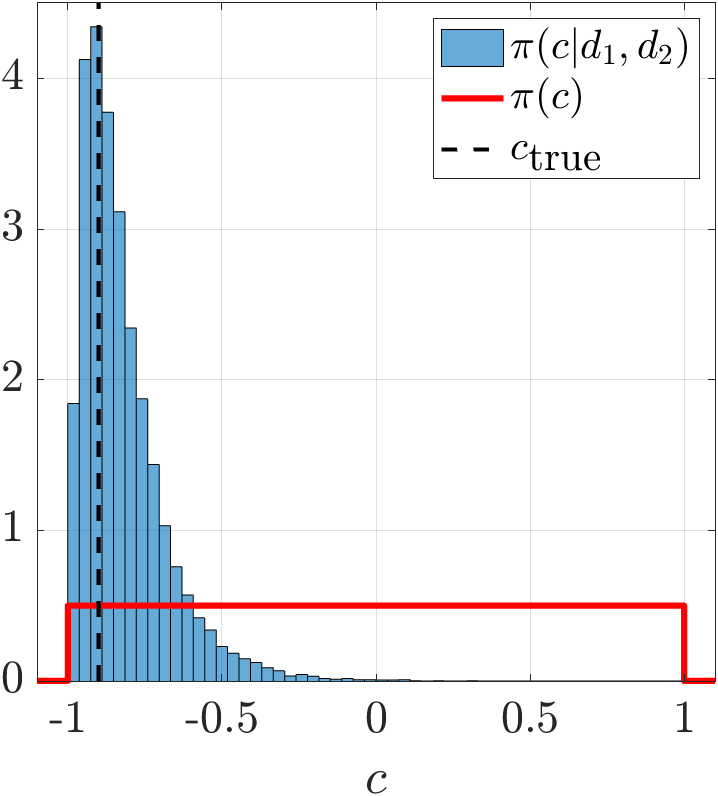
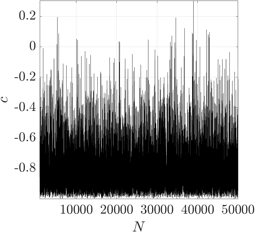
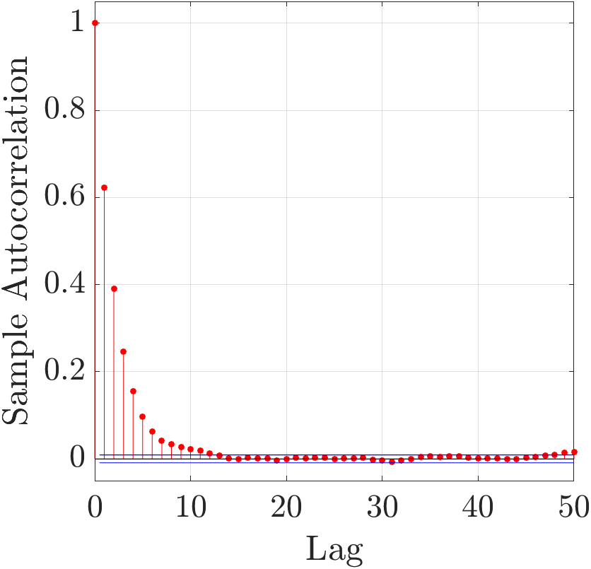
Figure 8: Posterior histogram and trace of the correlation estimate $\mathcal{N}(p_\ast, \Gamma_p)$8—the method places credible mass closely around the true value.

Example 2: Subsurface Flow with PDE Constraints

In a PDE-constrained inverse problem, log-permeability $\mathcal{N}(p_\ast, \Gamma_p)$9 and recharge $\mathcal{N}(m_\ast, \Gamma_m)$0 are inferred from head and direct $\mathcal{N}(m_\ast, \Gamma_m)$1 observations, allowing for spatially varying cross-correlation (two subdomains with different values of $\mathcal{N}(m_\ast, \Gamma_m)$2). As before, joint inference allows information transfer between parameters, particularly benefiting the field with weaker direct observation (here, recharge $\mathcal{N}(m_\ast, \Gamma_m)$3). The approach successfully recovers both subdomain correlations with credible posterior support, even in the presence of moderate nonlinearity.

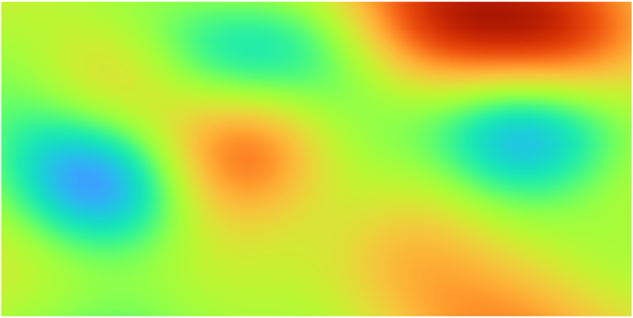
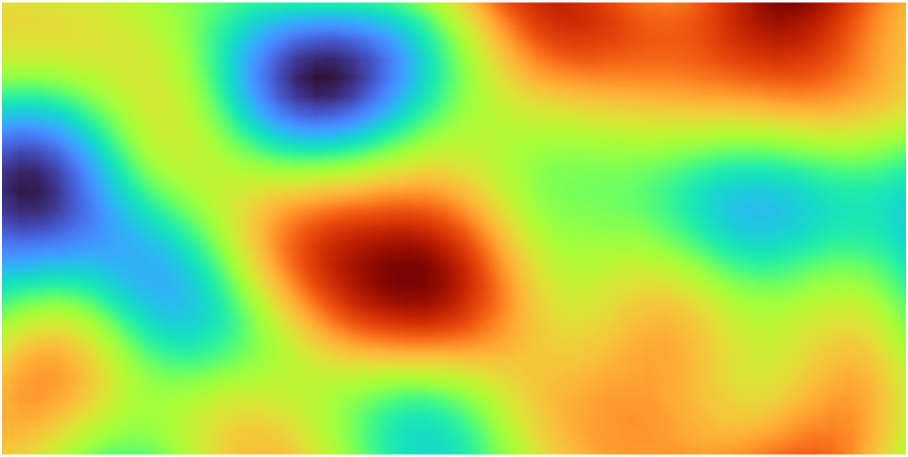
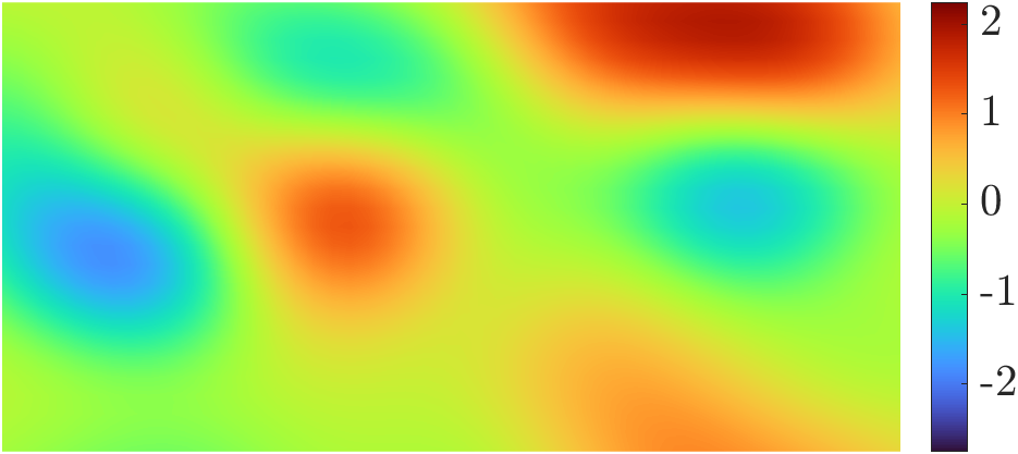
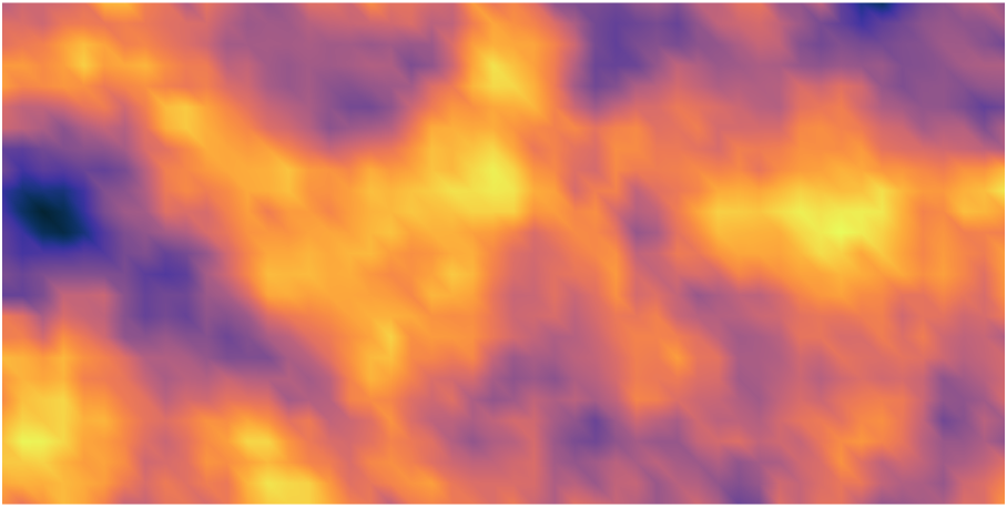
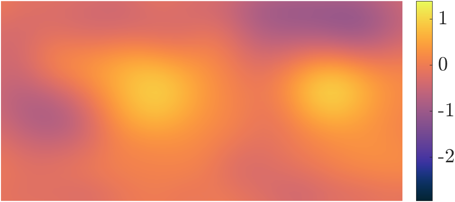
Figure 9: True fields and conditional mean estimates for log-permeability and log-recharge in the PDE-constrained inverse problem; error reductions are more pronounced in $\mathcal{N}(m_\ast, \Gamma_m)$4.

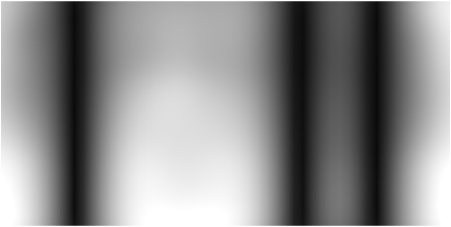
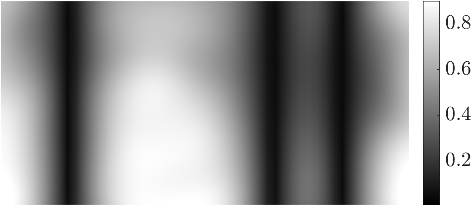
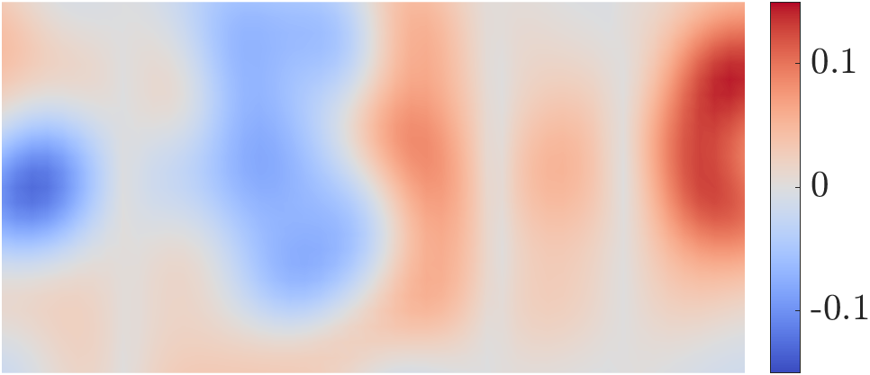
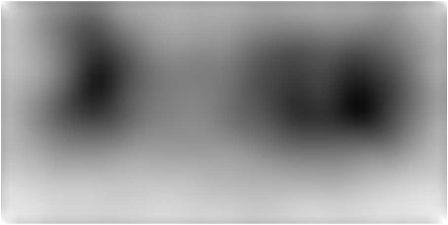
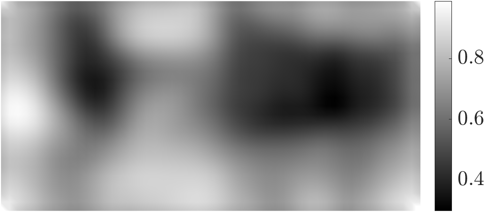
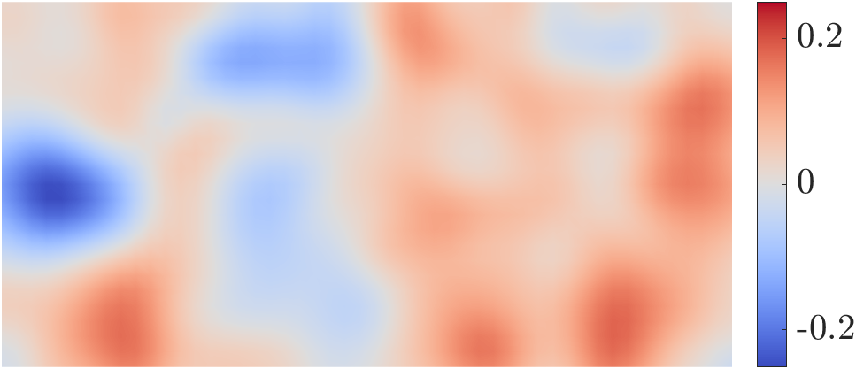
Figure 10: Marginal posterior standard deviations for $\mathcal{N}(m_\ast, \Gamma_m)$5 and $\mathcal{N}(m_\ast, \Gamma_m)$6—joint inference predominantly benefits $\mathcal{N}(m_\ast, \Gamma_m)$7, reflecting the indirect data structure.

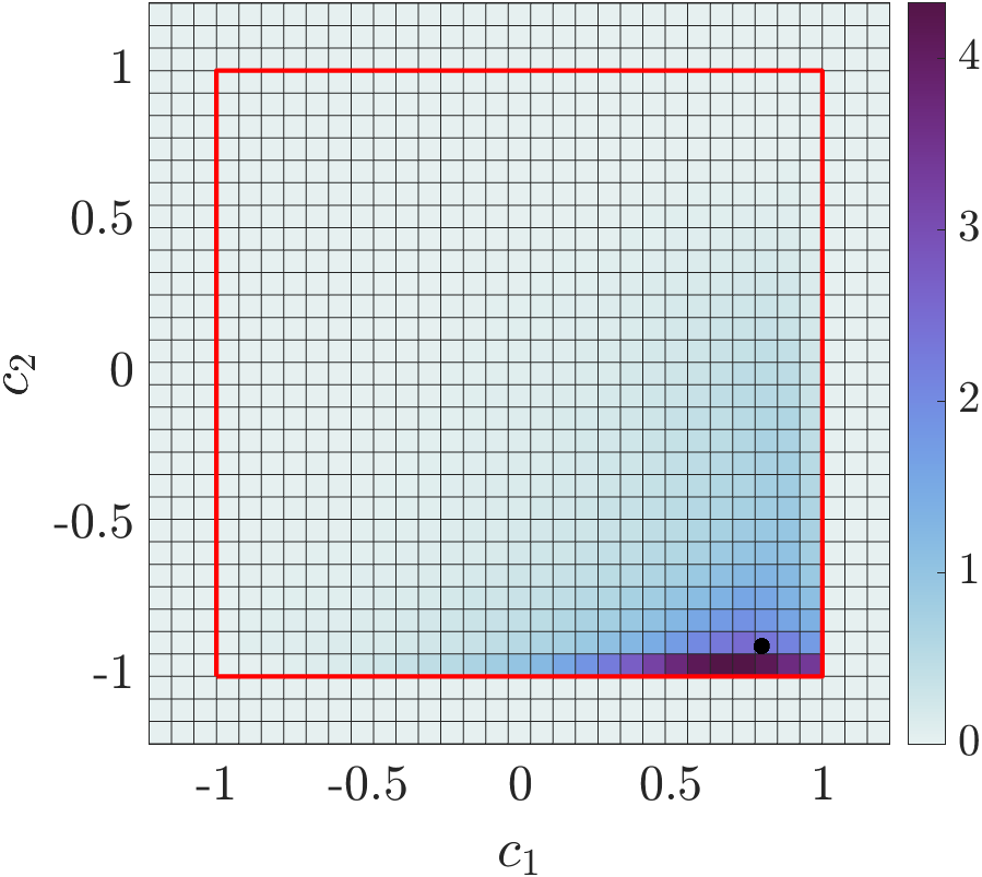
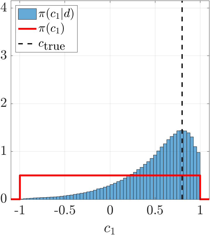
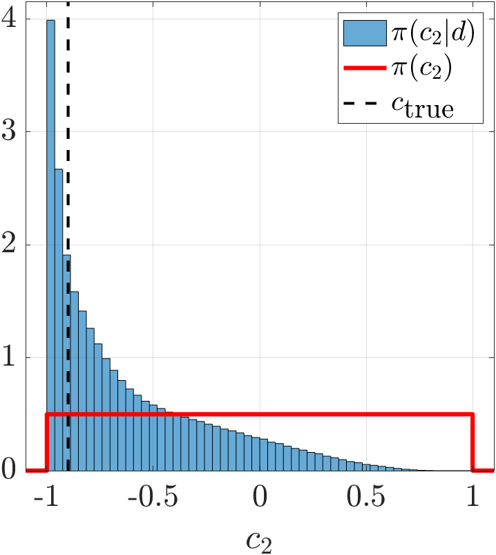
Figure 11: Marginal posteriors for the two regional correlations $\mathcal{N}(m_\ast, \Gamma_m)$8, reflecting the method’s ability to differentiate and infer piecewise-constant cross-correlations.

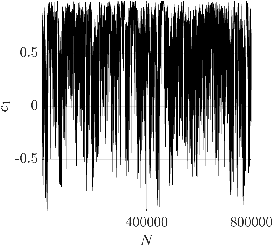
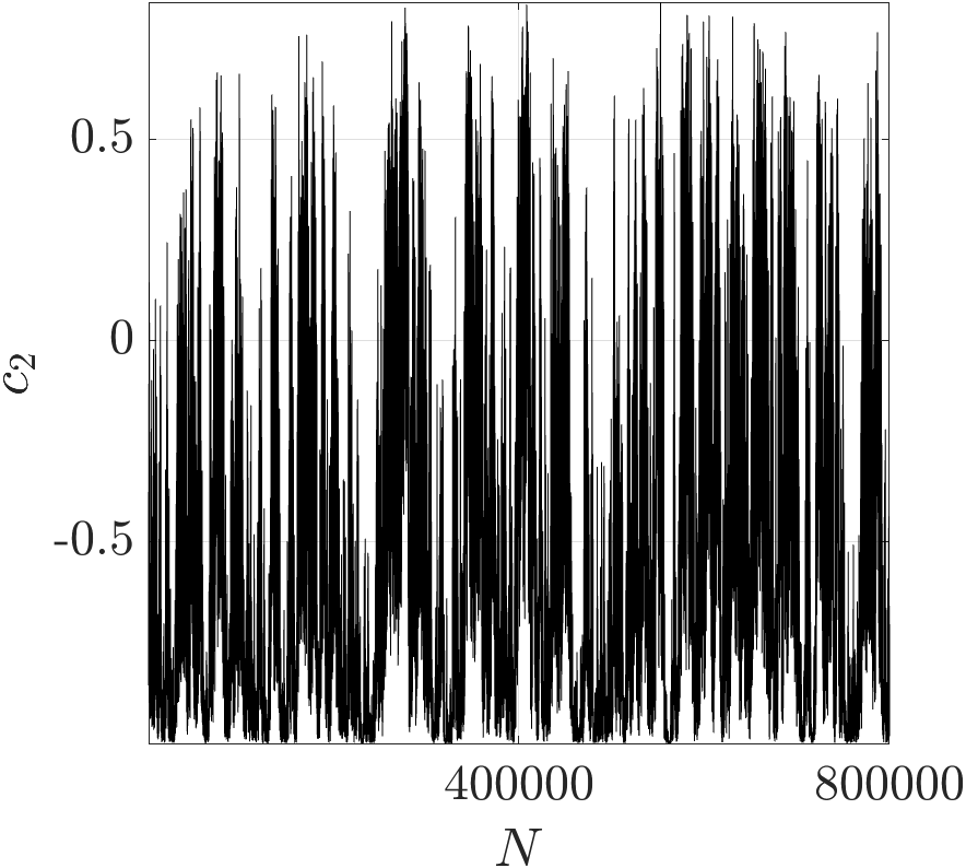
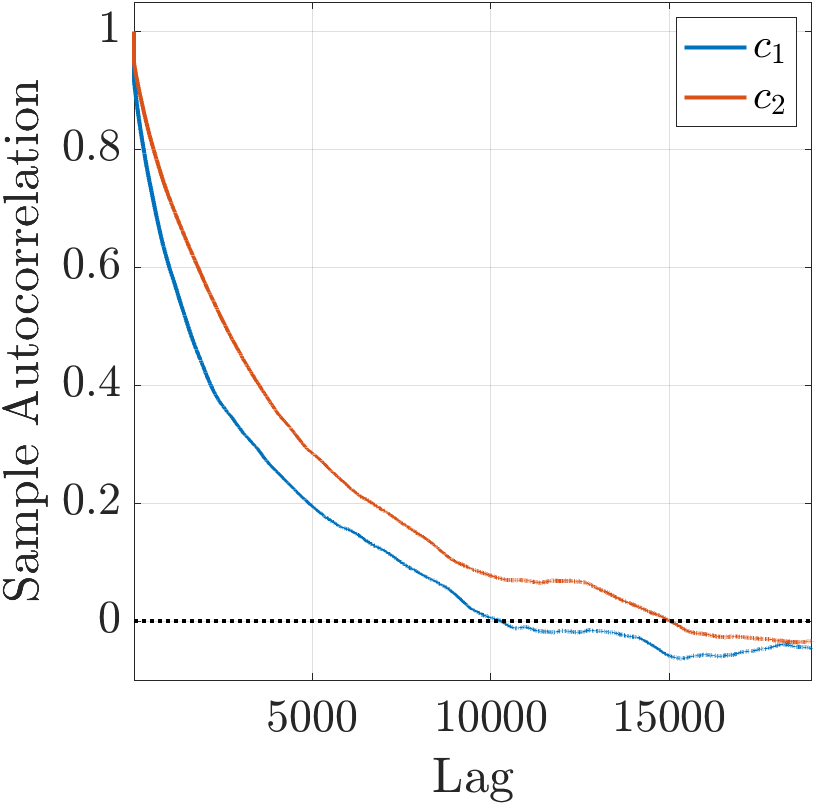
Figure 12: Diagnostics for MCMC chains on the correlation parameters, showing good exploration and moderate autocorrelation.

Implications, Limitations, and Future Directions

This framework fundamentally elevates the practice of joint Bayesian inversion by enabling both realistic prior modeling (preserving marginals while capturing arbitrary correlation) and coherent uncertainty propagation to all hyperparameters, including spatially varying correlation. Accounting for uncertainty in correlation avoids overconfident and potentially misleading posteriors encountered when enforcing independence or naive regularisation. It allows data to inform both the existence and spatial structure of relationships between fields.

However, the inclusion of hyperprior layers yields non-Gaussian posteriors requiring MCMC for characterisation, which increases computational cost and reduces effective sample size—particularly in high-dimensional or nonlinear settings. MAP-based approaches or Laplace approximation are generally not justified, often leading to pathological solutions (e.g., spurious maximisation at extreme correlation). While dimension reduction via Karhunen-Loève expansion mitigates some challenges, efficient sampling for hyperparameters in high dimension (potentially exploiting gradient-based samplers or variational inference) remains an open problem.

Conclusion

This work establishes a robust methodology for constructing and inferring jointly normal priors with prescribed marginals and tunable, spatially varying correlation operators in high-dimensional Bayesian inverse problems. The approach not only yields improved parameter estimation but also provides rigorous and interpretable quantification of uncertainty in both parameters and their mutual relationships—a requirement for applications where joint or co-structured field inference is indispensable. The results demonstrate that in any Bayesian model, unknowns—including correlation—must themselves be treated as random variables; failure to do so leads inevitably to erroneous uncertainty quantification and suboptimal inference.

Future research will address computational efficiency in posterior sampling for larger problems, alternative hyperprior parameterizations for structurally coupled fields (e.g., for level-set methods), and integration with gradient-based inference schemes to further facilitate practical deployment in large-scale multiphysics inversion.