An adaptive wavelet-based PINN for problems with localized high-magnitude source

Abstract: In recent years, physics-informed neural networks (PINNs) have gained significant attention for solving differential equations, although they suffer from two fundamental limitations, namely, spectral bias inherent in neural networks and loss imbalance arising from multiscale phenomena. This paper proposes an adaptive wavelet-based PINN (AW-PINN) to address the extreme loss imbalance characteristic of problems with localized high-magnitude source terms. Such problems frequently arise in various physical applications, such as thermal processing, electro-magnetics, impact mechanics, and fluid dynamics involving localized forcing. The proposed framework dynamically adjusts the wavelet basis function based on residual and supervised loss. This adaptive nature makes AW-PINN handle problems with high-scale features effectively without being memory-intensive. Additionally, AW-PINN does not rely on automatic differentiation to obtain derivatives involved in the loss function, which accelerates the training process. The method operates in two stages, an initial short pre-training phase with fixed bases to select physically relevant wavelet families, followed by an adaptive refinement that adapts scales and translations without populating high-resolution bases across entire domains. Theoretically, we show that under certain assumptions, AW-PINN admits a Gaussian process limit and derive its associated NTK structure. We evaluate AW-PINN on several challenging PDEs featuring localized high-magnitude source terms with extreme loss imbalances having ratios up to $10^{10}:1$. Across these PDEs, including transient heat conduction, highly localized Poisson problems, oscillatory flow equations, and Maxwell equations with a point charge source, AW-PINN consistently outperforms existing methods in its class.

• The paper introduces AW-PINN, a neural network that adapts wavelet bases for efficient and accurate handling of localized, high-magnitude source terms in multiscale PDEs.
• It employs a two-stage approach combining pre-training for wavelet family selection with adaptive refinement of scales and translations to focus representation on critical regions.
• Numerical experiments show significant error reductions and enhanced computational stability, supported by theoretical analysis via Gaussian process convergence and NTK decomposition.

Adaptive Wavelet-Based PINNs for Localized High-Magnitude Source Problems

Motivation and Limitations of PINNs in Multiscale and Imbalanced Scenarios

Physics-Informed Neural Networks (PINNs) have become a central paradigm for mesh-free solution of PDEs in forward and inverse settings due to their flexibility and compatibility with automatic differentiation. However, their efficacy breaks down in multiscale regimes and in the presence of large imbalances between loss components, such as problems containing highly localized, large-magnitude source terms. The spectral bias intrinsic to standard neural networks leads to rapid convergence on low-frequency solution features, impeding the learning of fast-varying phenomena. Loss imbalance, especially for extreme ratios (up to $10^{10}:1$ in the evaluated scenarios), further frustrates optimization, as the dominant components eclipse the relevant training signals for subtle solution features.

Classical approaches to resolving these challenges include spectral feature mapping (e.g., Fourier features), loss weighting or balancing (e.g., self-adaptive weights, exponent-regularized losses), and domain-specific architectures. While these methods partially mitigate pathology, they either require careful hyperparameter tuning, significant memory overhead, or they saturate for sufficiently extreme localization and scale disparity.

AW-PINN: Problem Statement and Architectural Innovations

The Adaptive Wavelet-based PINN (AW-PINN) introduces a hybrid approach that leverages wavelet bases as both representation and inductive bias, while making the basis adaptive—in both choice (family selection) and parameterization (scale and translation refinement)—according to problem-specific loss component analysis. The core concept is to restrict high-resolution wavelet basis functions to regions where the PDE’s structure and loss statistics necessitate them, as determined by data-driven similarity and alignment scores in a two-stage training process: pre-training/family selection and adaptive refinement.

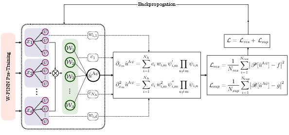
Figure 1: Schematic architecture of AW-PINN, showing initialization and optimization of wavelet units and linear output layer with adaptive scales and translations.

Pre-Training and Wavelet Family Selection

AW-PINN begins with a W-PINN-style initialization, spanning the computational domain with a rich set of wavelet basis functions at various dyadic scales and translations. Using pre-training (Adagrad/Adam plus shallow L-BFGS), the model identifies wavelet families with statistically significant alignment to both the PDE residuals and boundary/initial values (as reflected in large inner products of family response vectors with the source/condition data).

Only those basis functions above a similarity threshold or with the largest coefficients are retained. This pruning avoids the exponential blow-up in basis size and corresponding memory costs typical of full wavelet matrix approaches.

Adaptive Stage: Parameter Refinement and Analytical Derivatives

In the second stage, the chosen wavelet basis elements are “lifted” into parameterized wavelet units, whose scales and translations are now trainable variables. The architecture defines each adaptive wavelet unit as $$\mathcal{W}_i(\mathbf{x}; \theta_i) = \prod_{n=1}^d \psi(w_{i,n} x_n + b_{i,n})$$, with the initialization inherited from pre-training (e.g., $w_{i,n} = 2^{j_{i,n}}$, $b_{i,n} = -k_{i,n}$ for index $(j_{i,n}, k_{i,n})$).

A key technical component is the avoidance of automatic differentiation for loss term gradients: the implementation uses analytic expressions for all relevant derivatives, further lowering computational cost. The final network form is a sum over $N_\mathrm{A}$ adaptive wavelet units and a bias, with all parameters optimized via L-BFGS.

This architecture enables scale and location adaptation only in regions of physical or loss-driven interest, whereas traditional W-PINN methods assign high-resolution bases across the entire domain, leading to suboptimal scaling.

Theoretical Guarantees: Gaussian Process Limit and NTK Decomposition

The paper provides a rigorous analysis of AW-PINN’s representational properties and training dynamics in the infinite-width/infinite-family regime. Leveraging standard random feature model results, the output process of AW-PINN converges in law to a zero-mean Gaussian process $\mathcal{G}_p$ with kernel determined by expected correlations of random wavelet units. This result supports the view of AW-PINN as a kernel machine in the large-width limit, facilitating NTK-based analysis.

The empirical neural tangent kernel (NTK) splits into contributions from the linear weights $c_i$ and the adaptive parameters $(w_{i,n}, b_{i,n})$. Spectral properties of NTK (eigenvalue magnitudes and decay rates) govern the speed at which AW-PINN learns different solution features. The presence of adaptive scale/translation parameters enhances spectral flexibility relative to fixed W-PINN or standard PINN architectures.

Numerical Experiments: Quantitative and Qualitative Assessments

AW-PINN is assessed on a suite of challenging benchmark PDEs, each characterized by highly localized source terms or strong oscillatory behavior that induce extreme loss imbalance and/or multiscale solution structure.

1. Transient Heat Conduction with Extreme Source

A 1D parabolic equation with transient $\epsilon$-localized source and boundary/initial conditions produces loss ratios up to $$\mathcal{W}_i(\mathbf{x}; \theta_i) = \prod_{n=1}^d \psi(w_{i,n} x_n + b_{i,n})$$0. AW-PINN achieves relative $$\mathcal{W}_i(\mathbf{x}; \theta_i) = \prod_{n=1}^d \psi(w_{i,n} x_n + b_{i,n})$$1-errors on the order of $$\mathcal{W}_i(\mathbf{x}; \theta_i) = \prod_{n=1}^d \psi(w_{i,n} x_n + b_{i,n})$$2 over modest training times (20–25 min), outperforming W-PINN (errors $$\mathcal{W}_i(\mathbf{x}; \theta_i) = \prod_{n=1}^d \psi(w_{i,n} x_n + b_{i,n})$$3) and MMPINN (worse accuracy, higher time) and converging where baseline PINN fails.

(Figure 2)

Figure 2: Left to right: Heat source, AW-PINN prediction, and pointwise absolute error for the extreme-source heat problem.

AW-PINN achieves high accuracy with minimal local error and greater training stability compared to oscillatory error curves in MMPINN.

2. 2D Poisson Equation with Point-Wise Localization

Spatially sharp source terms lead to initial loss ratios of $$\mathcal{W}_i(\mathbf{x}; \theta_i) = \prod_{n=1}^d \psi(w_{i,n} x_n + b_{i,n})$$4. AW-PINN produces $$\mathcal{W}_i(\mathbf{x}; \theta_i) = \prod_{n=1}^d \psi(w_{i,n} x_n + b_{i,n})$$5-errors one to two orders of magnitude lower than MMPINN and W-PINN, with targeted adaptation of wavelet scales to the high-gradient region only, unlike W-PINN’s global high-resolution requirement.

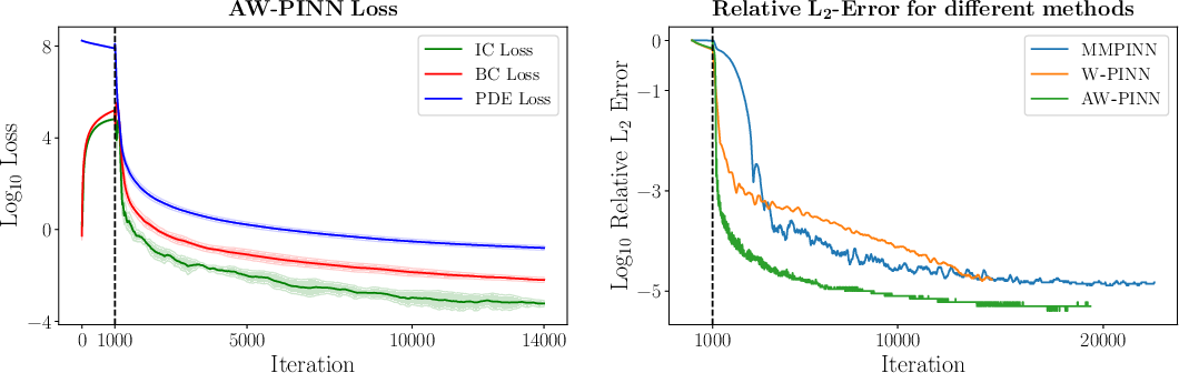
Figure 3: Source, ground-truth, AW-PINN prediction, and absolute errors for the Poisson localized-source problem.

(Figure 4)

Figure 4: Plots showing x- and y-scale adaptation in AW-PINN; adaptation is restricted to regions of high solution variation.

3. Flow Equations with Oscillating Source

For hyperbolic PDEs with oscillatory source terms, AW-PINN yields $$\mathcal{W}_i(\mathbf{x}; \theta_i) = \prod_{n=1}^d \psi(w_{i,n} x_n + b_{i,n})$$6-relative errors around $$\mathcal{W}_i(\mathbf{x}; \theta_i) = \prod_{n=1}^d \psi(w_{i,n} x_n + b_{i,n})$$7, a two-order-of-magnitude improvement over W-PINN and MMPINN.

(Figure 5)

Figure 5: Source, AW-PINN output, absolute errors, and time-slice predictions for the oscillatory-flow problem.

4. Maxwell's Equations with Point Charge

A coupled 3D system with a spatially and temporally localized point-source pulse challenges classic methods. AW-PINN consistently achieves low errors ($$\mathcal{W}_i(\mathbf{x}; \theta_i) = \prod_{n=1}^d \psi(w_{i,n} x_n + b_{i,n})$$8–$$\mathcal{W}_i(\mathbf{x}; \theta_i) = \prod_{n=1}^d \psi(w_{i,n} x_n + b_{i,n})$$9 in relative $w_{i,n} = 2^{j_{i,n}}$0 for all field components) in substantially less time than MMPINN, while baseline W-PINN and MMPINN perform poorly.

(Figure 6)

Figure 6: AW-PINN predictions and pointwise errors for in-plane electric and out-of-plane magnetic fields in Maxwell's equations setup.

Implications and Future Directions

The AW-PINN formulation addresses the limitations of mesh-free PINN methods for multiscale, strongly localized source-term PDEs in a scalable, theoretically grounded way. Its two-stage, similarity-driven adaptive basis selection balances representation economy with solution accuracy and provides explicit control over wavelet scale allocation. Analytic derivative evaluation and avoidance of autograd further enhance its computational efficiency for large-scale runs.

Practically, the method enables effective solution of ill-conditioned inverse and forward PDE problems encountered in areas such as thermal processing, electromagnetic modeling, impact mechanics, and advection-dominated flows. Theoretically, its convergence to a Gaussian process and the accompanying NTK structure allow precise study of learning dynamics and can permit new advances in architectural and optimization strategies tailored for PINNs.

Open issues remain: the semi-heuristic selection of relevant wavelet families depends on pre-training and requires parameter tuning. The integration of fully automated, potentially learning-theoretic selection criteria remains a promising avenue. Additionally, further systematic benchmarking over a broader class of problem types and exploration of alternative wavelet families are likely to refine the method’s generality and robustness.

Conclusion

AW-PINN presents a significant architectural and procedural advance for the efficient, stable, and accurate solution of PDEs with localized high-magnitude source terms, offering strong empirical and theoretical enhancements compared to prior multiscale and loss balancing approaches. By focusing adaptive representational power exactly where the physics and loss imbalance demand, it offers a compelling framework for future development of PINN-based solvers in scientific machine learning (2604.28180).