Generalization at the Edge of Stability
Abstract: Training modern neural networks often relies on large learning rates, operating at the edge of stability, where the optimization dynamics exhibit oscillatory and chaotic behavior. Empirically, this regime often yields improved generalization performance, yet the underlying mechanism remains poorly understood. In this work, we represent stochastic optimizers as random dynamical systems, which often converge to a fractal attractor set (rather than a point) with a smaller intrinsic dimension. Building on this connection and inspired by Lyapunov dimension theory, we introduce a novel notion of dimension, coined the `sharpness dimension', and prove a generalization bound based on this dimension. Our results show that generalization in the chaotic regime depends on the complete Hessian spectrum and the structure of its partial determinants, highlighting a complexity that cannot be captured by the trace or spectral norm considered in prior work. Experiments across various MLPs and transformers validate our theory while also providing new insights into the recently observed phenomenon of grokking.

Paper Prompts
Sign up for free to create and run prompts on this paper using GPT-5.
Top Community Prompts
Explain it Like I'm 14
What is this paper about?
This paper tries to explain why modern deep neural networks often work best when trained with big learning rates that make training unstable and even a bit chaotic. The authors show that, in this “edge of stability” zone, training doesn’t settle at one perfect set of weights. Instead, it wanders around a smaller, structured set of solutions. They introduce a new way to measure how complicated that set is, called the Sharpness Dimension (SD), and they prove that this number—not the total number of parameters—controls how well the model can generalize to new data.
The big questions
- Why do neural networks trained with large learning rates (where training can oscillate or look chaotic) often generalize better?
- Can we explain generalization by looking at the whole set of solutions the optimizer visits, rather than a single “final” solution?
- Is there a better complexity measure than just counting parameters or using simple Hessian-based “flatness/sharpness” scores?
How did the researchers study it?
To keep things simple, think of training like driving a car in a huge landscape (the “loss surface”). With small steps, you circle slowly toward a parking spot. With big steps, you might overshoot, skid, and end up looping around in a bounded area. That area is not random—it has structure.
Here are the main ideas, using everyday language:
- Random dynamical systems (RDS): Training with minibatches adds randomness to each step. You can think of the whole training process as a “system” that moves the weights around in time under random nudges. Mathematically, that’s an RDS.
- Attractors: Because of the randomness and the big steps, the process usually doesn’t settle at one point. Instead, it gets pulled into a set—the attractor—where it keeps moving but stays bounded. This set can be “fractal-like,” meaning complicated but lower-dimensional than the full parameter space.
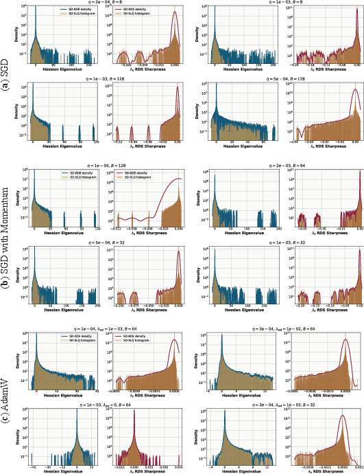
- Sharpness and the Hessian: The Hessian is a matrix that tells you how curved the loss surface is in all directions. Prior work often looked at only one number from it (like the biggest eigenvalue or the trace) as a proxy for “sharpness” or “flatness.” The authors argue that this is not enough—what matters is the whole spectrum (all curvatures in all directions).
- Sharpness Dimension (SD): The authors define a new measure, SD, inspired by Lyapunov/attractor dimensions from chaos theory. SD is built from how much training expands in some directions and contracts in others, averaged over the attractor. Intuitively:
- If training stretches space strongly in at least one direction (chaotic behavior), but still contracts overall, the optimizer explores a thinner, lower-dimensional set.
- The SD captures how many directions can keep “volume” from shrinking before contraction wins out.
- In the edge-of-stability regime, they show , where is the total number of parameters.
- Why “edge of stability” means chaos: When the largest local curvature (from the Hessian) goes beyond a certain threshold set by the learning rate, tiny differences in weights grow over time (a signature of chaos). This creates expansion in at least one direction—part of why the attractor has interesting, lower-dimensional structure.
What did they find and why is it important?
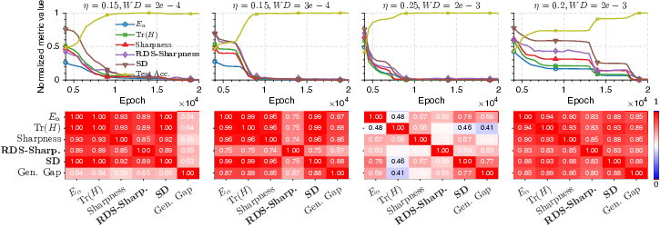
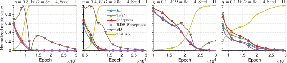
- A new generalization bound: They prove that the worst-case generalization error over the whole attractor is controlled by the Sharpness Dimension (SD). In plain terms: even if your model has millions of parameters, if the attractor your training runs on is effectively much lower-dimensional, your generalization can still be good—and the bound reflects that smaller SD.
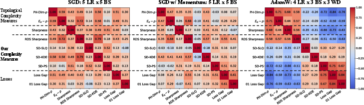
- Beyond simple sharpness: Their results depend on the complete Hessian spectrum (and specific combinations of it), not just a single number like the trace or the largest eigenvalue. This explains why earlier “flatness vs. sharpness” stories often fail—those summaries are too crude.
- Edge of stability is a good place to be: In the chaotic regime, they show the leading “sharpness” is positive (some directions expand), but overall the dynamics live on an attractor with . That lower effective dimension helps explain why big, overparameterized models can still generalize.
- Experiments back it up:
- On multilayer perceptrons (MLPs) and on a modern transformer (GPT‑2), their SD measure correlates well with real generalization performance—often better than standard sharpness/flatness measures or topological trajectory measures.
- They also study “grokking” (when a model suddenly starts to generalize after fitting the training data for a while). They find that changes in the Hessian spectrum and SD line up with this phase transition, offering a clearer picture of what’s happening under the hood.
What does this mean going forward?
- A clearer principle: Don’t judge a model’s generalization by parameter count or a single “flatness” number. Look at the effective dimensionality of the attractor the optimizer explores. If is small, generalization can be strong—even for very large models.
- Practical guidance:
- Training near the edge of stability isn’t just okay—it can be helpful, because it steers optimization onto a lower-dimensional, structured attractor.
- New diagnostics like SD (which the authors show how to estimate efficiently) can guide the choice of learning rates, batch sizes, and optimizers.
- Understanding grokking: The SD and full Hessian spectrum give a way to detect and interpret the sudden shift from memorization to generalization, helping researchers design training setups that encourage it.
In short, this work reframes generalization: it’s not about finding one flat minimum, but about the geometry of the entire set of solutions your training dynamics explore. The Sharpness Dimension captures that geometry and provides both a theory and a practical tool to understand—and improve—generalization in big, modern neural networks.
Knowledge Gaps
Knowledge gaps, limitations, and open questions
Below is a single, consolidated list of concrete gaps and unresolved questions that future work could address:
- Theoretical regularity gap: The analysis assumes – dynamics, bounded losses, and Lipschitz continuity, but many practical networks (e.g., ReLU/GeLU with layer norm, residuals) yield only piecewise-smooth, non– maps and use unbounded losses (e.g., cross-entropy). How can the framework be extended to non-smooth activations (e.g., via Clarke generalized Jacobians) and unbounded losses (e.g., via tail or truncation arguments)?
- Pullback attractor existence in practice: The existence of a bounded pullback absorbing set is assumed but not established for common deep architectures with ReLU, normalization, skip connections, and adaptive training heuristics. What verifiable sufficient conditions guarantee a compact pullback attractor for these cases?
- Non-singularity assumption: The theory requires the Jacobian to be non-singular (minimum singular value bounded away from 0) on the attractor, which is often violated in overparameterized networks with many flat directions. Can the results be extended to allow singular Jacobians (e.g., almost-everywhere non-singularity or stratified analysis)?
- Subexponential spatial variation (“bounded distortion”) assumption: There is no empirical or theoretical verification that the spatial variation of -volume growth rates is subexponential over real training attractors. Can this be tested, relaxed, or replaced with checkable conditions?
- Link to true Lyapunov spectrum: The “RDS sharpness” is defined via expected one-step log-singular values with a supremum over the attractor, not via products over time. Under what conditions does this quantity align with Oseledets/Lyapunov exponents, and how tight is the approximation in stochastic training?
- Equality/tightness of dimensions: The bound uses that the sharpness dimension upper-bounds the Minkowski (and relates to Hausdorff/Kaplan–Yorke) dimension. When do these dimensions coincide for random attractors arising in deep learning? Are there conditions guaranteeing tightness of the SD-based bound?
- Supremum over the attractor vs. point estimates: The definition uses , yet the estimation approximates SD at one or a few checkpoints. How can one reliably approximate the supremum over (e.g., via sampling along the attractor) and bound the resulting estimation error?
- Finite-sample estimation of SD: There is no formal sample-complexity or variance analysis for estimating SD via SLQ with minibatch Hessian–vector products. What is the bias/variance of SD estimates as a function of minibatch size, number of Lanczos runs, and mini-batch resampling?
- Minibatch vs. full-batch Hessian: The theory is expressed in terms of the true Jacobian/Hessian, but experiments use minibatch approximations. How sensitive is SD to replacing full-batch Hessians with minibatch ones, and can corrections or debiasing schemes be developed?
- Adaptive and momentum-based optimizers: The RDS formulation and Jacobian used in the theory are derived for (S)GD without momentum/adaptation, yet experiments include momentum and AdamW. How should the state-augmented dynamics (optimizer state + parameters) be modeled, and how does SD generalize in that enlarged state space?
- Time-varying training schedules: The framework targets stationary dynamics with persistent noise (constant learning rate). How can it be extended to non-stationary schedules (e.g., warm-up, cosine decay), where the map is explicitly time-dependent and the attractor may move or dissolve?
- Worst-case vs. typical generalization: The bound controls a worst-case gap over the attractor. In practice, evaluation is at a checkpoint or EMA/SWA average. Can one derive analogous bounds for time-averaged or stationary-distribution-weighted risks on the attractor?
- Dependence on parameterization: Like Hessian-based flatness measures, SD is likely not invariant to reparameterization or rescaling. What geometric (e.g., Fisher/natural-gradient) formulations make SD coordinate-invariant, and how do they compare empirically?
- Interpretability of “partial determinants”: The bound emphasizes dependence on products of singular values (partial determinants) rather than trace/spectral norm. Can one provide mechanistic interpretations and interventions (e.g., regularizers) targeting these products?
- Practical guidance for hyperparameter selection: Although correlations are reported, there are no actionable rules for choosing learning rate, batch size, weight decay, or optimizer to reduce SD and improve generalization. Can SD be used as an online hyperparameter signal?
- Role of data augmentation and stochasticity: The RDS can, in principle, include augmentation/dropout randomness, but experiments focus on minibatch noise. How does augmentation-induced noise change SD and the attractor’s dimension?
- Generalization bound constants and vacuity: The bound relies on constants and includes an term, but there is no discussion of magnitude or practical non-vacuity on real tasks. Can one provide non-asymptotic, numerically instantiated bounds and diagnose when they are informative?
- Handling the mutual information term : The bound includes , and its size is unknown. Can one upper-bound or replace it with computable set-stability quantities in common settings and verify its smallness empirically?
- Extension beyond classification on MNIST/modular arithmetic: Empirical validation is limited in scope (MNIST MLPs, grokking on small MLPs, and partial GPT-2). How does SD scale and correlate with generalization on larger vision models, large-scale LLMs, and diverse datasets?
- SD dynamics during training: Experiments suggest SD evolves and correlates with grokking, but there is no theoretical account predicting phase transitions or onset timing from SD. Can one model the temporal evolution of SD and link it causally to generalization phase transitions?
- Robustness and distribution shift: It remains unclear whether lower SD correlates with robustness to label noise, adversarial examples, or distribution shift. Can SD predict or control robustness properties?
- Interaction with flatness-based methods: How do explicit flatness regularizers (e.g., SAM, entropy-SGD, trace penalties) affect SD and the attractor? Are there cases where trace decreases but SD does not, and vice versa?
- Multiple attractors and multimodality: If the training dynamics admit multiple random attractors or metastable sets, how does the bound extend, and how should SD be aggregated across attractors?
- Finite-time vs. asymptotic gap: The analysis is asymptotic (attractor-based), but training and evaluation are finite-time. Can finite-time generalization guarantees be derived that interpolate between transient dynamics and attractor behavior?
- Architectural design for SD control: There is no guidance on how activation functions, normalization, residual connections, or depth/width influence SD. Can architecture-level prescriptions be derived to reduce SD without harming optimization?
- Thresholds for EoS and chaos: The link “ ⇒ EoS/chaos” is heuristic outside quadratics. Under what conditions does the largest Hessian eigenvalue exceeding imply positive top Lyapunov exponent in deep networks, and how does stochasticity alter this threshold?
Practical Applications
Immediate Applications
The paper’s findings enable several deployable uses that treat stochastic training as a random dynamical system (RDS), quantify complexity via Sharpness Dimension (SD), and exploit scalable estimation with stochastic Lanczos quadrature (SLQ).
- SD-driven training monitor and scheduler (software; NLP/vision/LLM fine-tuning; robotics)
- Use SD and the leading RDS sharpness λ₁ to monitor whether training is at the edge of stability (EoS), and auto-adjust learning rate, batch size, or momentum to keep λ₁>0 while minimizing SD.
- Tools/workflows: A PyTorch/JAX plugin that computes Hessian–vector products (HVPs) and estimates the SD from minibatches via SLQ; integrated with schedulers (e.g., to damp LR when SD spikes, or increase LR when SD is too low and overfitting persists).
- Assumptions/dependencies: Efficient HVPs are available; SLQ estimation variance is manageable with minibatch-based Hessian approximations; training operates in or near EoS; additional compute overhead is acceptable.
- Hyperparameter selection, early stopping, and checkpointing by SD (industry/academia; AutoML)
- Rank runs and checkpoints by SD rather than Hessian trace alone; stop training when SD plateaus or begins to rise; select the checkpoint with the lowest SD consistent with target training loss.
- Tools/workflows: Add SD to run dashboards (e.g., WandB) and AutoML search objectives; store SD in checkpoints for post-hoc selection.
- Assumptions/dependencies: Loss and its gradient/HVPs remain stable across epochs for consistent SD estimation; data and optimization noise are representative of deployment.
- Generalization diagnostics beyond trace/flatness (industry/academia)
- Diagnose why two runs with similar Hessian traces generalize differently by comparing full-spectrum SD; identify regimes where traditional “flatness” surrogates fail but SD discriminates.
- Tools/workflows: SD vs. generalization plots across seeds/β (momentum)/weight decay; per-layer or blockwise SD analyses to spot problematic modules.
- Assumptions/dependencies: SLQ reliably captures the bulk spectrum (including near-zero modes) relevant for SD; loss is Lipschitz-bounded enough for the bound’s qualitative guidance.
- Grokking phase-transition detection (academia; LLM/MLP training)
- Track SD/λ₁ to anticipate or characterize the onset of grokking (delayed sudden generalization); adjust weight decay or LR schedules to accelerate or stabilize grokking.
- Tools/workflows: SD curves over training epochs with alerts on sudden inflection points; dashboards comparing SD to train/test gaps.
- Assumptions/dependencies: Grokking setups exhibit EoS-like dynamics; SD estimation at sparse checkpoints captures the phase transition.
- LLM fine-tuning guardrails (software; NLP)
- During GPT-2–scale fine-tuning, estimate SD via minibatch HVP+SLQ to choose learning-rate, batch-size, and weight-decay settings that keep SD low while maintaining λ₁>0.
- Tools/workflows: Hugging Face Accelerate + PyTorch functorch VJP/JVP HVPs; asynchronous SLQ during logging intervals; checkpoint selection by SD.
- Assumptions/dependencies: HVP throughput on available hardware is sufficient; SLQ runs do not unduly slow training; minibatch Hessians approximate full-batch curvature adequately.
- Stability-aware online learning in robotics and control (robotics)
- Use SD/λ₁ as a real-time stability indicator for on-device adaptation; reduce step size or freeze layers when SD spikes, preventing brittle updates while preserving adaptation speed.
- Tools/workflows: Lightweight HVPs over recent minibatches; threshold-based controller to gate updates.
- Assumptions/dependencies: Compute budget permits periodic HVPs; data distribution during deployment is close to training; safety constraints tolerate brief pauses for stability checks.
- Risk-sensitive model development in healthcare and finance (healthcare; finance)
- Use SD thresholds as additional acceptance criteria for models trained on small/noisy datasets; prefer configurations with lower SD at fixed empirical risk to curb overfitting.
- Tools/workflows: Compliance checklists including SD; model cards including SD-based complexity summaries; cross-validation runs ranked by SD.
- Assumptions/dependencies: Domain losses and metrics satisfy bounded/Lipschitz assumptions approximately; additional compute for SD is feasible under regulatory timelines.
- Evaluating optimizers and regularizers by SD (academia/industry)
- Compare SGD, momentum, AdamW, SAM, SWA, and weight decay settings by their induced SD (not just loss/accuracy), guiding selections toward methods that reduce SD while preserving performance.
- Tools/workflows: Benchmark suites logging SD across optimizers and seeds; ablation studies on curvature shaping.
- Assumptions/dependencies: Optimizer implementations expose HVPs without extensive modification; SD is estimated consistently across methods.
Long-Term Applications
The results also suggest new methods and infrastructure that will require further research, scaling, or engineering.
- SD-regularized optimizers and objectives (software; academia)
- Develop optimizers that directly control the partial-volume expansion terms underlying SD (e.g., penalize the sum of log top-j singular values of I−ηH, or regularize partial determinants) to shape attractor geometry.
- Tools/products/workflows: New training objectives and regularizers approximating SD gradients via HVP-based surrogates; proximal updates that constrain expansion directions.
- Assumptions/dependencies: Tractable proxies for SD gradients exist with acceptable variance; regularization does not unduly harm optimization; further theory for non-smooth nets/Adam-like updates.
- Architecture search with SD as a complexity objective (software; AutoML)
- Incorporate SD into neural architecture search (NAS) to prefer modules/activations that yield lower SD for target tasks, improving generalization at scale.
- Tools/products/workflows: NAS pipelines with periodic SD probes; per-block SD attribution to guide design (e.g., normalization, activation choices).
- Assumptions/dependencies: SD can be estimated quickly enough during NAS; SD correlates with deployment metrics across architectures and datasets.
- Scalable SD estimation for frontier models (software/hardware)
- Design distributed SLQ, sketching, or low-rank-plus-diagonal approximations for full-spectrum SD estimation in billion-parameter models; hardware primitives for high-throughput HVPs.
- Tools/products/workflows: Multi-GPU/TPU SLQ libraries; kernel fusion for HVP; compiler support for repeated VJP/JVP.
- Assumptions/dependencies: Communication costs do not dominate; approximations preserve SD fidelity; vendor support for second-order ops.
- SD-guided pruning and quantization (software; energy efficiency)
- Use SD to identify expansion-prone directions/modules; prune or quantize to reduce SD while maintaining accuracy, yielding models that generalize better with smaller footprints.
- Tools/products/workflows: Layerwise SD diagnostics; structured pruning that targets high-expansion subspaces; post-quantization SD checks.
- Assumptions/dependencies: Causal links between SD reductions and robust accuracy hold across tasks; pruning/quantization pipelines can access reliable SD signals.
- Federated and continual learning with attractor control (software; mobile/edge; healthcare)
- Control global/local attractor complexity across clients by constraining SD, preventing instability under heterogeneous data; use SD to schedule updates and memory consolidation.
- Tools/products/workflows: Client-side SD measurements; server aggregation that penalizes clients with high SD; curriculum over clients/tasks.
- Assumptions/dependencies: Communication of SD (or proxies) is privacy-preserving; client HVPs are feasible; heterogeneous losses still comply with bounded/Lipschitz approximations.
- Data curation and active learning via spectrum shaping (academia/industry)
- Select or weight training examples to shape the Hessian spectrum and reduce SD, improving generalization with fewer labels.
- Tools/products/workflows: Influence-function or gradient-covariance estimates to predict SD impact of samples; active learning loops targeting SD reduction.
- Assumptions/dependencies: Reliable mapping from data selection to Hessian spectrum exists; cost of spectral feedback fits labeling budgets.
- Safety and regulatory standards using SD-based bounds (policy; high-stakes domains)
- Establish reporting standards requiring SD tracking and SD-based generalization certificates in sensitive domains (e.g., clinical models).
- Tools/products/workflows: Auditable training logs including SD trajectories; bound-based risk disclosures alongside performance metrics.
- Assumptions/dependencies: Community consensus on acceptable SD thresholds; further empirical validation linking SD to safety outcomes across modalities.
- Theory extensions and guarantees for modern training (academia)
- Extend bounds to non-smooth activations (ReLU), adaptive optimizers (AdamW), non-stationary data, and non-Lipschitz losses; relate SD to robustness and calibration.
- Tools/products/workflows: New RDS analyses incorporating momentum/Adam; empirical process tools adapted to SD; benchmarks spanning modalities.
- Assumptions/dependencies: Existence of random pullback attractors in broader settings; bounded-distortion-like conditions for practical optimizers.
- RL and control: chaos-aware policy optimization (robotics; reinforcement learning)
- Use SD to stabilize policy optimization where chaotic updates hamper generalization and safety; enforce SD constraints during trust-region or actor-critic updates.
- Tools/products/workflows: SD-augmented TRPO/PPO; scheduling entropy/learning rates based on SD signals.
- Assumptions/dependencies: HVP access for policy networks; online SD estimation with acceptable latency in control loops.
Cross-cutting assumptions and dependencies
- The practical bound and many applications presume: bounded and (approximately) Lipschitz losses; C² dynamics for the optimizer; non-singularity and integrability on attractors; subexponential bounded distortion. Deviations (e.g., sharp non-Lipschitzities, heavy-tailed noise) may weaken guarantees or the stability of SD estimates.
- SD estimation requires efficient Hessian–vector products and sufficient minibatch averaging; compute overhead must be budgeted, especially for large models.
- Benefits are most pronounced in regimes near the edge of stability; if training is far from EoS (very small learning rates), SD may be less informative than simpler metrics.
- For high-stakes deployment, SD should complement, not replace, domain-specific validation and robustness testing.
Glossary
- alpha-weighted lifetime sum: A topological statistic from persistent homology that aggregates feature lifetimes with an exponent α to summarize trajectory geometry. "Topological summaries such as the `-weighted lifetime sum' exhibit consistent correlations with the generalization gap across training runs \citep{andreeva2024topological, tuci2025mutual}."
- bounded distortion: An assumption that the variation of volume growth rates across points on the attractor is subexponential in time, ensuring uniform leading-order expansion/contraction. "We assume that the spatial variation of over the attractor is subexponential in :"
- chaos: Dynamical behavior exhibiting sensitive dependence on initial conditions; in this context, positive expansion rates lead to chaotic training dynamics. "\citet{ly2025optimization} demonstrated that exceeding the threshold of is sufficient to induce chaotic training dynamics."
- cocycle: A time-indexed family of maps over a base dynamical system satisfying a consistency (composition) property; here it encodes optimizer updates over noise. "satisfies the cocycle property:"
- edge of stability (EoS): The regime where training operates near the stability threshold, often with oscillatory/chaotic dynamics and improved generalization. "This behavior, termed the edge of stability (EoS), has generated considerable interest"
- forward-invariant set: A set mapped into itself by the dynamics, providing a bounded region preventing divergence even at large learning rates. "the existence of a forward-invariant set prevents divergence"
- fractal attractor set: A complex, often self-similar limit set of the dynamics with non-integer effective dimension, rather than a single point. "which often converge to a fractal attractor set (rather than a point) with a smaller intrinsic dimension."
- Gaussian quadrature: A numerical integration technique used here within stochastic Lanczos methods to recover spectral densities. "followed by Gaussian quadrature and kernel smoothing."
- grokking: A phenomenon where models suddenly generalize after prolonged training despite earlier overfitting. "providing new insights into the recently observed phenomenon of grokking."
- Hausdorff semi-distance: A measure of set distance capturing how far points of one set are from the other, used in defining pullback attraction. "is the Hausdorff semi-distance."
- Hessian spectrum: The collection of eigenvalues of the Hessian; its full structure influences generalization in the proposed theory. "depends on the complete Hessian spectrum"
- Hessian trace: The sum of Hessian eigenvalues; a common flatness proxy linking curvature to generalization. "most practical surrogates rely on second-order cues such as the trace of the Hessian"
- invariant measure: A probability measure preserved by the dynamics; for SGD under contraction, the invariant measure can live on a fractal set. "stochastic GD (SGD) admits an invariant measure supported on a fractal set"
- Jacobian: The derivative (matrix) of the update map; its singular values/eigenvalues determine local expansion and stability. "The local stability of this system is governed by the Jacobian ."
- Kendall's coefficients: Rank-correlation measures (e.g., Kendall’s τ) used to assess monotonic relationships between complexity and generalization. "We assess the correlation between various notions of complexity and generalization error by using Kendall's coefficients (KC)"
- Krylov-based methods: Iterative linear-algebra techniques (e.g., Lanczos) for spectral estimation that can struggle with clustered near-zero spectra. "Krylov-based methods such as Lanczos iterations~\cite{lanczos1950iteration} become ineffective."
- left-shift operator: A shift map on the sequence of random seeds/minibatch indices advancing the noise history in RDS formulations. "the so-called the `left-shift operator',"
- Lyapunov dimension theory: A framework connecting Lyapunov exponents to fractal dimensions of attractors; it motivates the sharpness dimension. "inspired by Lyapunov dimension theory,"
- Lyapunov exponent: The asymptotic exponential rate of separation of nearby trajectories; positivity indicates chaos. "the top Lyapunov exponent see \citet[Lemma~3.2.2, p.~113]{arnold2006random} becomes positive ."
- metric dynamical system: A probability space with a measure-preserving, ergodic transformation providing the base flow for an RDS. "A metric dynamical system "
- mini-batch sharpness: A stability proxy based on curvature measured with respect to mini-batch gradients during SGD. "via the notion of mini-batch sharpness"
- Minkowski dimension: A fractal dimension defined via covering numbers; here it is upper-bounded by the sharpness dimension. "another notion of fractal dimension called the Minkowski dimension"
- mutual information (total mutual information): An information-theoretic quantity capturing dependence between the dataset and the learned (random) attractor. "denotes the total mutual information between the random pullback attractor and ."
- partial determinants: Products of leading singular values (or eigenvalues), representing j-volume expansion; these structure the role of curvature beyond trace/norm. "and the structure of its partial determinants"
- pullback random attractor: A noise-conditioned invariant set obtained by evolving from the distant past; the central object capturing long-run behavior under randomness. "is called a pullback random attractor"
- random dynamical system (RDS): A dynamical system driven by stochastic inputs/noise, modeling stochastic optimizers like SGD. "A discrete-time random dynamical system (RDS) on is a tuple"
- RDS Sharpness: A global expansion measure defined via expected log singular values of the Jacobian over the attractor. "We define the RDS Sharpness of Order "
- sharpness dimension (SD): A dimension-like complexity derived from ordered expansion rates (sharpness indices), quantifying the attractor’s effective dimensionality. "coined the `sharpness dimension'"
- spectral norm: The largest singular value of a matrix; a curvature/complexity proxy contrasted with trace in prior work. "highlighting a complexity that cannot be captured by the trace or spectral norm considered in prior work."
- stability threshold (2/η): The gradient-descent stability limit for quadratic approximations; exceeding it leads to instability/chaos. "the threshold implies instability and divergence for quadratic objectives"
- stochastic Lanczos quadrature (SLQ): A scalable method combining Lanczos iterations with quadrature to estimate spectral densities. "we adopt stochastic Lanczos quadrature (SLQ)"
Collections
Sign up for free to add this paper to one or more collections.

