Physics-Informed Neural Networks: A Didactic Derivation of the Complete Training Cycle

Abstract: This paper is a step-by-step, self-contained guide to the complete training cycle of a Physics-Informed Neural Network (PINN) -- a topic that existing tutorials and guides typically delegate to automatic differentiation libraries without exposing the underlying algebra. Using a first-order initial value problem with a known analytical solution as a running example, we walk through every stage of the process: forward propagation of both the network output and its temporal derivative, evaluation of a composite loss function built from the ODE residual and the initial condition, backpropagation of gradients -- with particular attention to the product rule that arises in hidden layers -- and a gradient descent parameter update. Every calculation is presented with explicit, verifiable numerical values using a 1-3-3-1 multilayer perceptron with two hidden layers and 22 trainable parameters. From these concrete examples, we derive general recursive formulas -- expressed as sensitivity propagation relations -- that extend the gradient computation to networks of arbitrary depth, and we connect these formulas to the automatic differentiation engines used in practice. The trained network is then validated against the exact solution, achieving a relative $L^2$ error of $4.290 \times 10^{-4}$ using only the physics-informed loss, without any data from the true solution. A companion Jupyter/PyTorch notebook reproduces every manual calculation and the full training pipeline, providing mutual validation between hand-derived and machine-computed gradients.

• The paper presents a complete didactic derivation of both forward and backward passes in PINNs, meticulously outlining the gradient computation process.
• The paper demonstrates that hand-derived recursive sensitivity formulas align exactly with automatic differentiation outputs, ensuring transparent and verifiable training dynamics.
• The paper validates a 1-3-3-1 MLP PINN achieving a relative L² error of 4.290×10⁻⁴, underscoring effective loss balancing between ODE residuals and initial conditions.

Didactic Derivation and Validation of the Complete Physics-Informed Neural Network Training Cycle

Introduction and Motivation

"Physics-Informed Neural Networks: A Didactic Derivation of the Complete Training Cycle" (2604.18481) addresses a fundamental gap in the scientific machine learning literature—the explicit articulation, at a granular algebraic level, of the forward and backward passes constituting PINN training. Existing resources, both introductory and advanced, routinely outsource these details to automatic differentiation libraries, thus obscuring the parameter-dependent gradients necessitated by embedding physical laws within the loss. This work provides, step-by-step and with hand-verifiable numerical values, the complete forward and backward computations for a PINN trained to solve a prototypical ODE: $y'(t) + y(t) = 0$ with initial condition $y(0) = 1$, utilizing a modest 1-3-3-1 MLP architecture.

The didactic clarity is paired with a rigorous validation of the PINN approach: the model is trained exclusively on a physics-informed composite loss, with no access to ground-truth solution data, and yields a relative $L^2$ error of $4.290 \times 10^{-4}$ with only 22 parameters. The mechanistic exposition is complemented by general recursive formulas that are directly connected to modern autodiff engines.

PINN Architecture and Forward Pass

The central modeling setup is a feedforward neural network with one input ($t$), two hidden layers of three neurons each, and one output, resulting in a 1-3-3-1 MLP footprint. Hidden layers use $\tanh$ (both nonlinearity and differentiability requirements), and the output layer is linear, as required by regression tasks.

The overall training cycle is structured as follows: initialization, dual forward propagation (simultaneous computation of both $\hat{y}$ and $\hat{y}'$ at collocation points and the initial condition), composite loss evaluation, backpropagation (gradient computation w.r.t. all parameters), and parameter update.

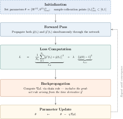
Figure 1: Four-stage training cycle for PINNs, visualizing initialization, dual forward pass, loss computation, gradient backpropagation with explicit product rule handling, and parameter update.

A single artificial neuron operates via standard affine transformation followed by nonlinearity, but, critically for PINNs, its activation function must be at least twice differentiable even for first-order ODE losses, as the product rule in the backward pass introduces second derivatives.

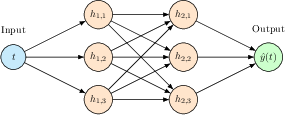
Figure 2: 1-3-3-1 MLP architecture, highlighting the dimensions and calculation of trainable parameters per layer.

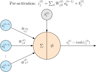
Figure 3: Elementwise operation of an artificial neuron, with affine transformation and non-linear activation, whose derivatives are analytically traced through the network.

In the forward pass, the composite loss consists of the ODE residual loss, $L_R$, evaluated at collocation points, and the initial condition loss, $L_{IC}$, weighted by a hyperparameter $y(0) = 1$0. Both $y(0) = 1$1 and its temporal derivative $y(0) = 1$2 are propagated through each layer; the latter is necessary since physical loss constraints involve derivatives w.r.t. input.

Algebraic Structure of Backpropagation in PINNs

Distinct from vanilla deep learning, PINN backpropagation for physical residuals requires parameter gradients of both the network output and its input derivative. For hidden layers, this incurs additional product rule terms: parameters affect not only the value but also the derivative of activations, propagating sensitivity through both standard and temporal paths.

The authors provide full backward passes for all parameter types, e.g., for output weights, the gradient is a sum of partials:

$y(0) = 1$3

For hidden weights, both the usual chain rule through successive layers and product rule terms (involving $y(0) = 1$4) appear, corresponding precisely to the parameter’s influence on $y(0) = 1$5 and $y(0) = 1$6 via multiple paths.

Generalizing, two recursively computed sensitivities are propagated forward: $y(0) = 1$7 (activation sensitivity) and $y(0) = 1$8 (time-derivative sensitivity), for every neuron $y(0) = 1$9 at every layer $L^2$0, initialized according to the parameter type (weight or bias) being differentiated. These recursions, together with the final summing at the output, provide fully general formulas for any classic feedforward PINN.

This explicit symbolic structure exactly mirrors what autograd engines compute, and the included code confirms the exact match of manual and library-computed gradients.

Training Dynamics and Empirical Validation

Under standard stochastic optimization (Adam, $L^2$1) and with 30 uniformly spaced collocation points, the network is trained for 15,000 epochs. A clear two-phase convergence is observed: first, the initial condition is rapidly satisfied (due to strong $L^2$2 weighting), and then training focuses on minimizing the ODE residual $L^2$3 throughout the interval.

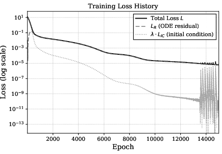
Figure 4: Log-scale evolution of total loss $L^2$4, ODE residual $L^2$5, and initial condition loss $L^2$6 over 15,000 epochs, illustrating rapid initial condition satisfaction and subsequent ODE residual minimization.

Solution quality is assessed against the analytical $L^2$7 at 500 evaluation points. The PINN’s predictions are nearly indistinguishable from the analytic solution, with a maximum absolute error of $L^2$8 and a relative $L^2$9 error of $4.290 \times 10^{-4}$0.

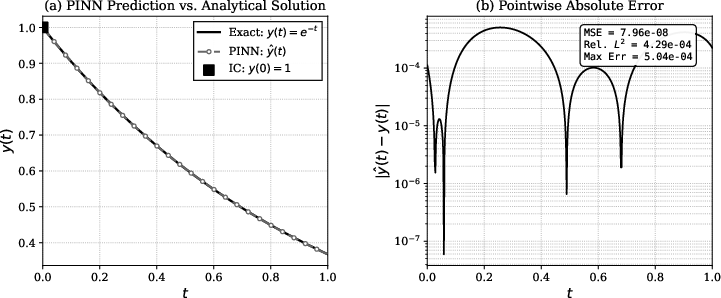
Figure 5: PINN prediction and pointwise absolute error compared to the analytic solution $4.290 \times 10^{-4}$1, showing sub-$4.290 \times 10^{-4}$2 errors across the domain.

The analyzed training dynamics reveal that weighting (i.e., the $4.290 \times 10^{-4}$3 hyperparameter) introduces multi-phase convergence and competition between physics and initial/boundary constraints, as documented in the modern PINN literature.

Theoretical and Practical Implications

The detailed gradient structure clarified by this derivation has several consequences:

• Product rule requirement for hidden parameter gradients: The necessity of evaluating second derivatives of activations even for first-order problems dictates activation function choice for PINNs, in contrast to standard DL settings.
• Direct connection to autodiff engine mechanics: The recursive sensitivity propagation for both value and temporal derivative demonstrates how autodiff frameworks handle higher-order, parameter-dependent derivatives in internally consistent fashion.
• Emphasis on hyperparameter tuning (loss balancing): The fact that initial condition enforcement and PDE residual minimization interact nontrivially is numerically and conceptually evident, leading to open questions on loss weight selection, curriculum schedules, and adaptive strategies.
• Foundations for generalizations: While the test problem is simple, the recursive sensitivity framework is directly extensible to networks of greater depth and to more complex PDEs, setting the stage for methodologies addressing high-dimensional domains, inverse problems, and data assimilation.
• Pedagogical and implementation transparency: The explicit connection between hand-derived computations and machine autodiff is invaluable for both educational purposes and the verification of codes applied to research and industrial PINN deployments.

Future Directions

The explicit derivations and general formulas naturally extend to:

• Higher-order ODEs and multidimensional PDEs, where multiple derivatives and where tensor-valued parameters amplify sensitivity recursion complexity and interaction effects.
• Studies of training dynamics under various optimizer and activation function regimes, including the handling of pathological gradient flows (as recently observed in deep PINNs) and the applicability of second-order or meta-learning-based optimizers.
• Inverse and parametric PINNs, as the derivation holds when physical coefficients themselves are treated as network parameters.

Conclusion

The work unpacks, in complete analytic detail, the forward and backward computational graph of a multi-layer PINN, exposing structure often hidden by high-level autodiff libraries. The empirical results demonstrate that a physics-informed loss, even with minimal network capacity and without reference to solution data, achieves highly accurate function approximation. Most critically, the recursive sensitivity relations support straightforward generalization to deep PINNs and complex physical constraints, anchoring both further research and robust implementation.

This didactic approach enables clearer theoretical inquiry into gradient pathologies, activation design, and multitask loss balancing, and will likely facilitate method development for larger-scale, physically-constrained models in scientific machine learning and engineering.