GS-STVSR: Ultra-Efficient Continuous Spatio-Temporal Video Super-Resolution via 2D Gaussian Splatting

Abstract: Continuous Spatio-Temporal Video Super-Resolution (C-STVSR) aims to simultaneously enhance the spatial resolution and frame rate of videos by arbitrary scale factors, offering greater flexibility than fixed-scale methods that are constrained by predefined upsampling ratios. In recent years, methods based on Implicit Neural Representations (INR) have made significant progress in C-STVSR by learning continuous mappings from spatio-temporal coordinates to pixel values. However, these methods fundamentally rely on dense pixel-wise grid queries, causing computational cost to scale linearly with the number of interpolated frames and severely limiting inference efficiency. We propose GS-STVSR, an ultra-efficient C-STVSR framework based on 2D Gaussian Splatting (2D-GS) that drives the spatiotemporal evolution of Gaussian kernels through continuous motion modeling, bypassing dense grid queries entirely. We exploit the strong temporal stability of covariance parameters for lightweight intermediate fitting, design an optical flow-guided motion module to derive Gaussian position and color at arbitrary time steps, introduce a Covariance resampling alignment module to prevent covariance drift, and propose an adaptive offset window for large-scale motion. Extensive experiments on Vid4, GoPro, and Adobe240 show that GS-STVSR achieves state-of-the-art quality across all benchmarks. Moreover, its inference time remains nearly constant at conventional temporal scales (X2--X8) and delivers over X3 speedup at extreme scales X32, demonstrating strong practical applicability.

• The paper introduces GS-STVSR, leveraging 2D Gaussian Splatting to achieve ultra-efficient continuous spatio-temporal video super-resolution by bypassing the computational bottlenecks of traditional Implicit Neural Representation (INR) methods.
• GS-STVSR capitalizes on the robust temporal stability of 2D Gaussian covariance parameters, enabling a lightweight convolutional model for covariance transitions and focusing computational capacity on accurate position and color estimation.
• The framework achieves state-of-the-art reconstruction quality with superior inference speed (up to 5x faster than BF-STVSR) and fewer parameters, making it highly suitable for real-time video processing across various applications.
• The framework introduces a Covariance Resampling Alignment (CRA) module to predict stable intermediate covariances and an Optical Flow-Guided Continuous Gaussian Motion Learning module for robust position and color parameter generation, complemented by a Motion-Aware Adaptive Offset Window (AOW) for handling large-scale motions.

GS-STVSR: Ultra-Efficient Continuous Spatio-Temporal Video Super-Resolution via 2D Gaussian Splatting

Continuous Spatio-Temporal Video Super-Resolution (C-STVSR) represents a crucial advancement in video processing, aiming to enhance both spatial resolution and frame rate by arbitrary factors. Recent methods relying on Implicit Neural Representations (INRs), such as VideoINR (2604.18047), MoTIF (2604.18047), and BF-STVSR (2604.18047), have made significant strides in C-STVSR by modeling continuous mappings from spatio-temporal coordinates to pixel values. However, these INR-based approaches suffer from a fundamental limitation: their reliance on dense pixel-wise grid queries leads to computational costs that scale linearly with the number of interpolated frames, severely hindering inference efficiency and practicability.

The GS-STVSR framework addresses these limitations by leveraging 2D Gaussian Splatting (2D-GS), an ultra-efficient representation that bypasses dense grid queries entirely. This work introduces a novel approach that drives the spatio-temporal evolution of 2D Gaussian kernels through continuous motion modeling. The core insight underpinning GS-STVSR is the robust temporal stability of Gaussian covariance parameters. Experimental analysis demonstrates that these parameters exhibit a temporal correlation of approximately 0.99 between adjacent frames, significantly surpassing the correlation observed in the pixel domain. This inherent stability allows for the use of lightweight convolutional operations to model covariance transitions, thereby focusing the model’s capacity on the more intricate tasks of position and color estimation.

The GS-STVSR framework comprises three key components (Figure 1): a Covariance Resampling Alignment (CRA) module, an Optical Flow-Guided Continuous Gaussian Motion Learning module, and a Motion-Aware Adaptive Offset Window (AOW).

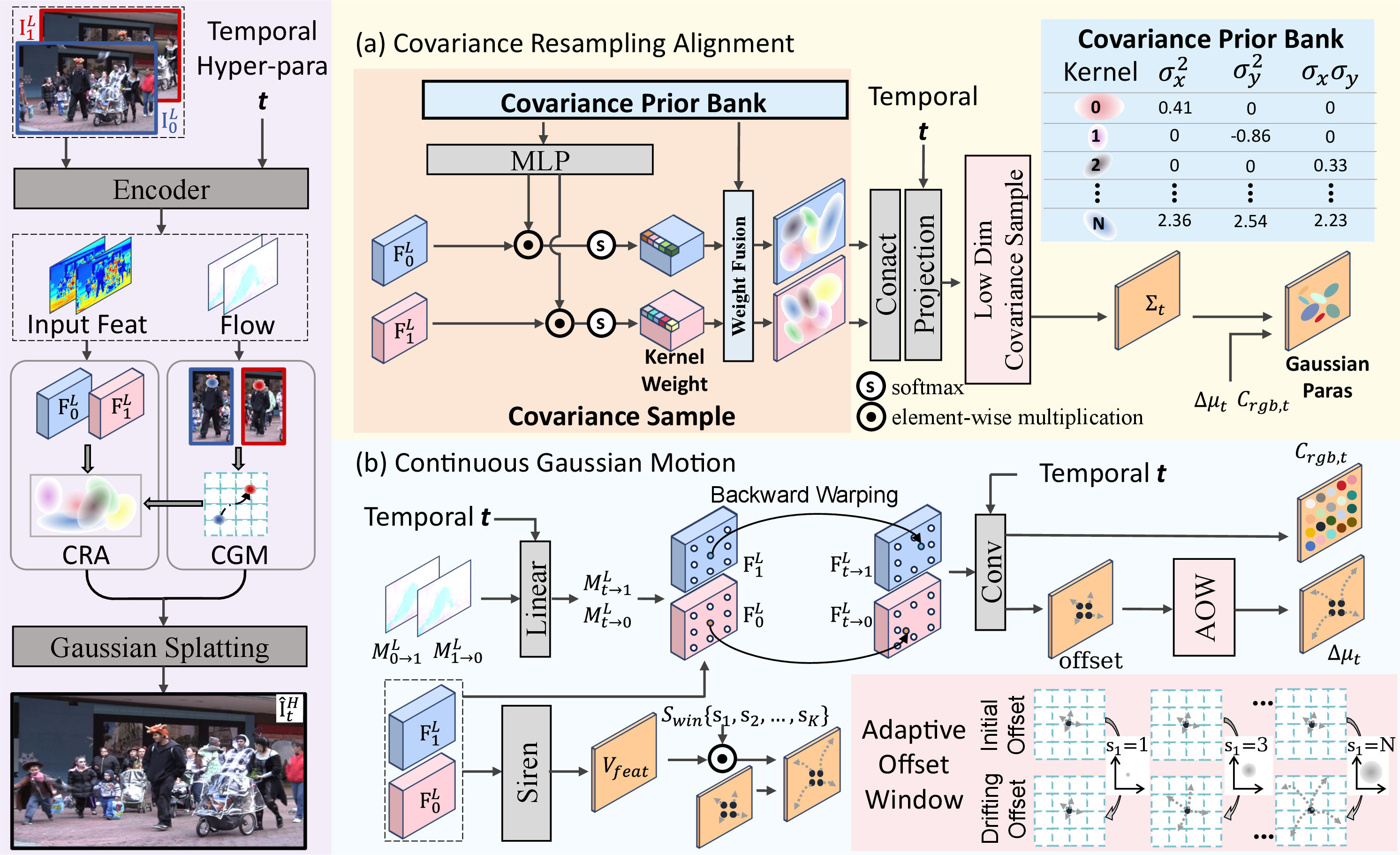
Figure 1: Overview of the GS-STVSR framework. Given two low-resolution frames, features and bidirectional optical flows are extracted. Gaussian parameter estimation is decoupled into two branches: (a) The Covariance Resampling Alignment Module predicts intermediate covariance by resampling from a Covariance Prior Bank (CPB) to ensure temporal stability; (b) The Continuous Gaussian Motion Learning Module uses optical flows for feature backward warping to estimate color and position, with a Motion-Aware Adaptive Offset Window (AOW) adjusting position offset based on local motion intensity. Finally, complete Gaussian parameters are combined with the target spatial scale for fast 2D Gaussian Splatting rasterization.

Covariance Resampling Alignment Module

The Covariance Resampling Alignment module is designed to predict intermediate covariance parameters ($\Sigma_t$) effectively and stably. Initial endpoint covariances ($\Sigma_0, \Sigma_1$) are derived from deep features by sampling from a pre-defined Covariance Prior Bank (CPB). The observed temporal stability of covariance parameters, as quantitatively demonstrated by high Pearson Correlation Coefficient and Cosine Similarity values compared to pixel-domain values (Figure 2), is leveraged.

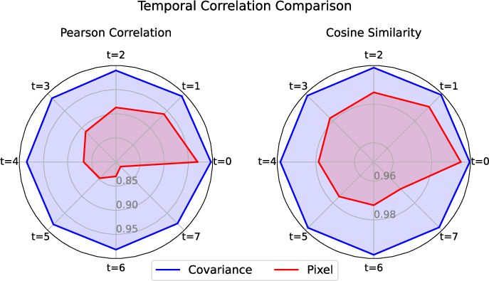
Figure 2: Comparison of temporal correlation between pixel-level and covariance-based representations. The radar charts evaluate the correlation across continuous time intervals (t=0 to 7) using Pearson Correlation (left) and Cosine Similarity (right). Gaussian covariance (blue) exhibits significantly higher and more stable temporal consistency than raw pixels (red).

This stability suggests that complex non-linear transformations are unnecessary for covariance transition. Consequently, $\Sigma_t$ is predicted via a single-layer convolution on the concatenation of $\Sigma_0$, $\Sigma_1$, and the target time $t$. To prevent covariance drift, where unbounded convolutions might push $\Sigma_t$ off the CPB manifold, the convolution output is compressed into a low-dimensional fusion feature. This feature then acts as adaptive sampling weights over the CPB, enabling a weighted re-combination to obtain $\Sigma_t$, thereby anchoring it within the CPB manifold and ensuring stability with minimal computational overhead.

Optical Flow-Guided Continuous Gaussian Motion Learning

The generation of position ($\Delta \mu_t$) and color ($C_{rgb,t}$) parameters at arbitrary time $\Sigma_0, \Sigma_1$0 is achieved through an optical flow-guided motion learning module. This module eschews the MLP-based parameter generation of prior 2D-GS techniques, which would introduce substantial computational costs due to per-frame MLP inferences. Instead, pre-extracted bidirectional optical flows ($\Sigma_0, \Sigma_1$1) provide explicit motion guidance. Intermediate optical flows are derived via linear scaling under a short inter-frame interval assumption. Endpoint deep features are then warped to the target time $\Sigma_0, \Sigma_1$2 using these intermediate flows. A lightweight convolution module processes the warped features to predict an adaptive spatio-temporal fusion mask and a feature residual, compensating for potential alignment errors caused by the linear motion assumption, particularly around occlusion boundaries. The fused feature is then decoded by a lightweight convolutional head to produce $\Sigma_0, \Sigma_1$3 and $\Sigma_0, \Sigma_1$4. This design maximizes efficiency by sharing optical flow computation across time steps, with only minimal time-dependent overheads for fusion and decoding.

Motion-Aware Adaptive Offset Window

A significant challenge in extending 2D-GS to video is the handling of large inter-frame motions. Traditional 2D-GS approaches often constrain position offsets to a local pixel grid for stability, which is inadequate for dynamic video content where Gaussian kernels must shift substantially along trajectories. Preliminary experiments confirmed that a naive global relaxation of the offset window degrades performance in static regions. The Motion-Aware Adaptive Offset Window (AOW) addresses this by dynamically adjusting the offset range based on local motion intensity. A weight map is learned from endpoint features and combined with predefined base windows to yield a spatially varying window map. This map scales the initial position offset prediction, allowing wider offset ranges in areas of significant motion while maintaining tight regularization in static regions (Figure 3). This adaptive mechanism enables accurate trajectory tracking for large-scale motions and mitigates multi-frame overlapping artifacts, which are evident in the absence of AOW (Figure 4).

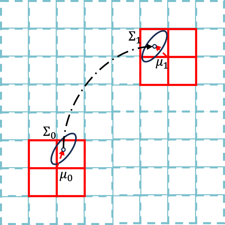
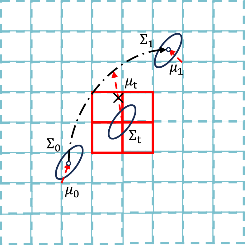
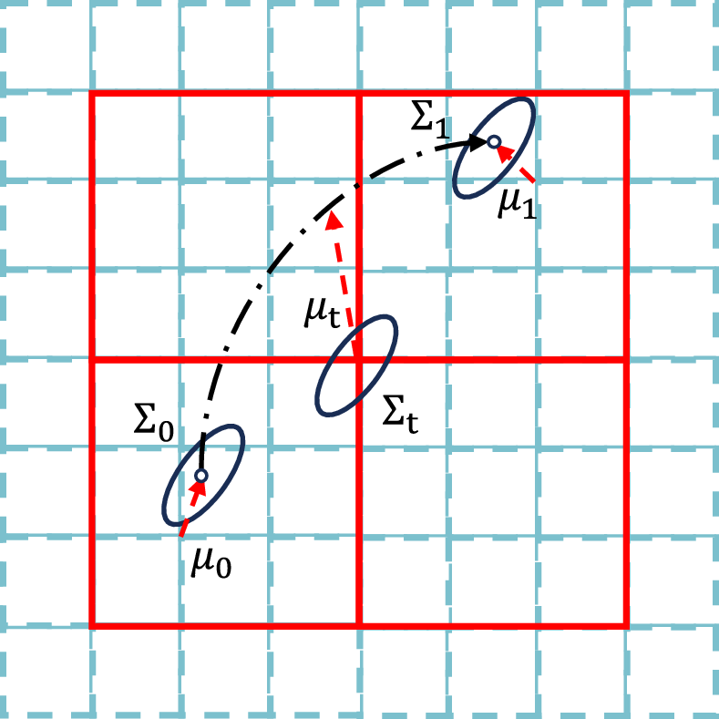
Figure 3: Illustration of the Motion-Aware Adaptive Offset Window under large-scale motion. (a) Possible trajectories between endpoint frames. (b) A small offset window provides insufficient range to reach the actual trajectory. (c) An appropriately large offset window ensures accurate trajectory targeting.

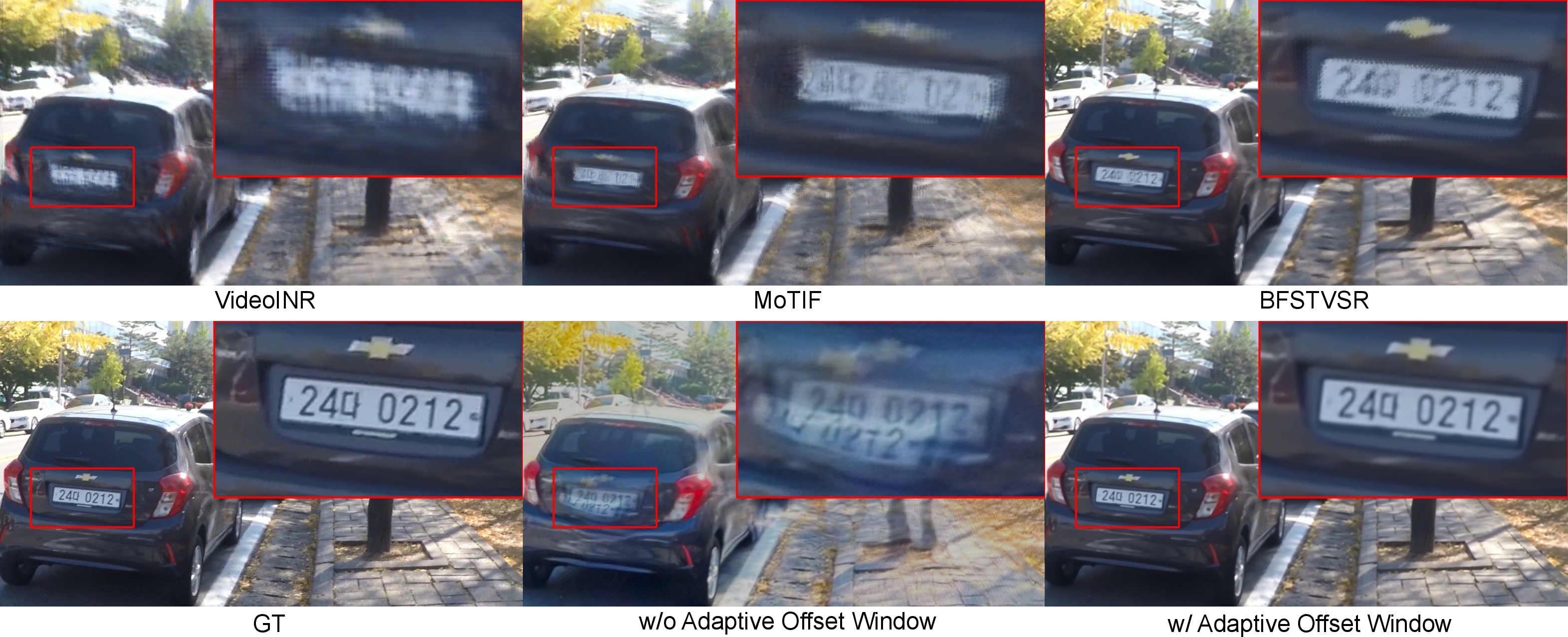
Figure 4: Visual comparison at t = 0.5 on a GoPro test scene with large camera shake (times 4 spatial, times 8 temporal).

Experimental Results

GS-STVSR demonstrates state-of-the-art performance across multiple benchmarks, including Vid4, GoPro, and Adobe240 datasets. Quantitative results show that GS-STVSR consistently achieves the highest PSNR and SSIM scores across all five F-STVSR evaluation settings, outperforming BF-STVSR, while utilizing fewer parameters (12.67M vs. 13.47M) (Table 1).

Table 1: Performance comparison on the F-STVSR baselines on Vid4, GoPro, and Adobe240 datasets (PSNR (dB) / SSIM in Y channels).

VFI Method	VSR Method	Vid4	GoPro-Center	GoPro-Average	Adobe-Center	Adobe-Average	Parameters (M)	AT (s)
SuperSloMo	Bicubic	22.42 / 0.5645	27.04 / 0.7937	26.06 / 0.7720	26.09 / 0.7435	25.29 / 0.7279	19.8	-
SuperSloMo	EDVR	23.01 / 0.6136	28.24 / 0.8322	26.30 / 0.7960	27.25 / 0.7972	25.90 / 0.7682	19.8+20.7	-
SuperSloMo	BasicVSR	23.17 / 0.6159	28.23 / 0.8308	26.36 / 0.7977	27.28 / 0.7961	25.94 / 0.7679	19.8+6.3	-
QVI	Bicubic	22.11 / 0.5498	26.50 / 0.7791	25.41 / 0.7554	25.57 / 0.7324	24.72 / 0.7114	29.2	-
QVI	EDVR	23.48 / 0.6547	28.60 / 0.8417	26.64 / 0.7977	27.45 / 0.8087	25.64 / 0.7590	29.2+20.7	-
QVI	BasicVSR	23.15 / 0.6428	28.55 / 0.8400	26.27 / 0.7955	26.43 / 0.7682	25.20 / 0.7421	29.2+6.3	-
DAIN	Bicubic	22.57 / 0.5732	26.92 / 0.7911	26.11 / 0.7740	26.01 / 0.7461	25.40 / 0.7321	24.0	-
DAIN	EDVR	23.48 / 0.6547	28.58 / 0.8417	26.64 / 0.7977	27.45 / 0.8087	25.64 / 0.7590	24.0+20.7	-
DAIN	BasicVSR	23.43 / 0.6514	28.46 / 0.7966	26.43 / 0.7966	26.23 / 0.7725	25.23 / 0.7725	24.0+6.3	-
ZoomingSloMo		25.72 / 0.7717	30.69 / 0.8847	- / -	30.26 / 0.8821	- / -	11.10	-
TMNet		25.96 / 0.7803	30.14 / 0.8696	28.83 / 0.8514	29.41 / 0.8524	28.30 / 0.8354	12.26	5.67
VideoINR		25.61 / 0.7709	30.26 / 0.8792	29.41 / 0.8669	29.92 / 0.8746	29.27 / 0.8651	11.31	3.34
MoTIF		25.79 / 0.7745	31.04 / 0.8877	30.04 / 0.8773	30.63 / 0.8839	29.82 / 0.8750	12.55	1.77
BF-STVSR		25.85 / 0.7772	31.17 / 0.8898	30.22 / 0.8802	30.83 / 0.8880	30.12 / 0.8808	13.47	1.27
Ours		26.04 / 0.7822	31.33 / 0.8918	30.35 / 0.8817	31.13 / 0.8907	30.35 / 0.8827	12.67	0.64

Furthermore, GS-STVSR exhibits superior generalization to out-of-distribution spatio-temporal scales (Table 2), with performance advantages becoming more pronounced at increasing scales.

Table 2: Performance comparison on the C-STVSR baselines for out-of-distribution scale on GoPro dataset (PSNR (dB) / SSIM in Y channels).

Temporal Scale	Spatial Scale	RIFE + LIIF	RIFE + LTE	EMA-VFI + LIIF	EMA-VFI + LTE	VideoINR	MoTIF	BF-STVSR	Ours
×8	×4	29.14 / 0.8524	29.14 / 0.8524	29.68 / 0.8671	29.68 / 0.8667	29.41 / 0.8669	30.04 / 0.8773	30.22 / 0.8802	30.33 / 0.8815
	×4	30.16 / 0.8738	30.16 / 0.8737	30.64 / 0.8850	30.64 / 0.8848	30.75 / 0.8978	31.53 / 0.9060	31.71 / 0.9082	31.83 / 0.9092
×6	×6	27.87 / 0.8038	27.86 / 0.8031	28.17 / 0.8126	28.17 / 0.8117	28.37 / 0.8368	29.25 / 0.8499	29.33 / 0.8514	29.39 / 0.8517
	×12	24.74 / 0.7019	24.70 / 0.6994	24.85 / 0.7052	24.82 / 0.7028	24.55 / 0.7126	25.62 / 0.7310	25.56 / 0.7276	25.74 / 0.7341
	×4	27.43 / 0.8102	27.42 / 0.8100	27.90 / 0.8263	27.90 / 0.8260	27.36 / 0.8174	27.73 / 0.8222	28.08 / 0.8287	28.18 / 0.8303
×12	×6	26.19 / 0.7640	26.19 / 0.7636	26.49 / 0.7748	26.49 / 0.7743	26.14 / 0.7795	26.68 / 0.7897	26.96 / 0.7955	27.10 / 0.7979
	×12	24.03 / 0.6869	24.00 / 0.6853	24.16 / 0.6918	24.15 / 0.6902	23.58 / 0.6902	24.56 / 0.7088	24.68 / 0.7084	24.88 / 0.7155
	×4	26.08 / 0.7735	26.08 / 0.7733	26.56 / 0.7904	26.56 / 0.7902	25.76 / 0.7738	25.93 / 0.7745	26.40 / 0.7839	26.53 / 0.7866
×16	×6	25.24 / 0.7394	25.24 / 0.7391	25.54 / 0.7503	25.55 / 0.7499	25.01 / 0.7473	25.24 / 0.7513	25.71 / 0.7611	25.85 / 0.7642
	×12	23.57 / 0.6781	23.56 / 0.6769	23.68 / 0.6828	23.69 / 0.6816	23.00 / 0.6762	23.73 / 0.6903	24.04 / 0.6936	24.23 / 0.7009

Qualitative results (Figure 5, Figure 6, Figure 7, Figure 8, Figure 9, Figure 10) further demonstrate that GS-STVSR produces visually superior frames with sharper details, clearer structural boundaries, and fewer motion artifacts compared to existing INR-based methods, even under challenging conditions involving fast-moving objects or mutual occlusions.

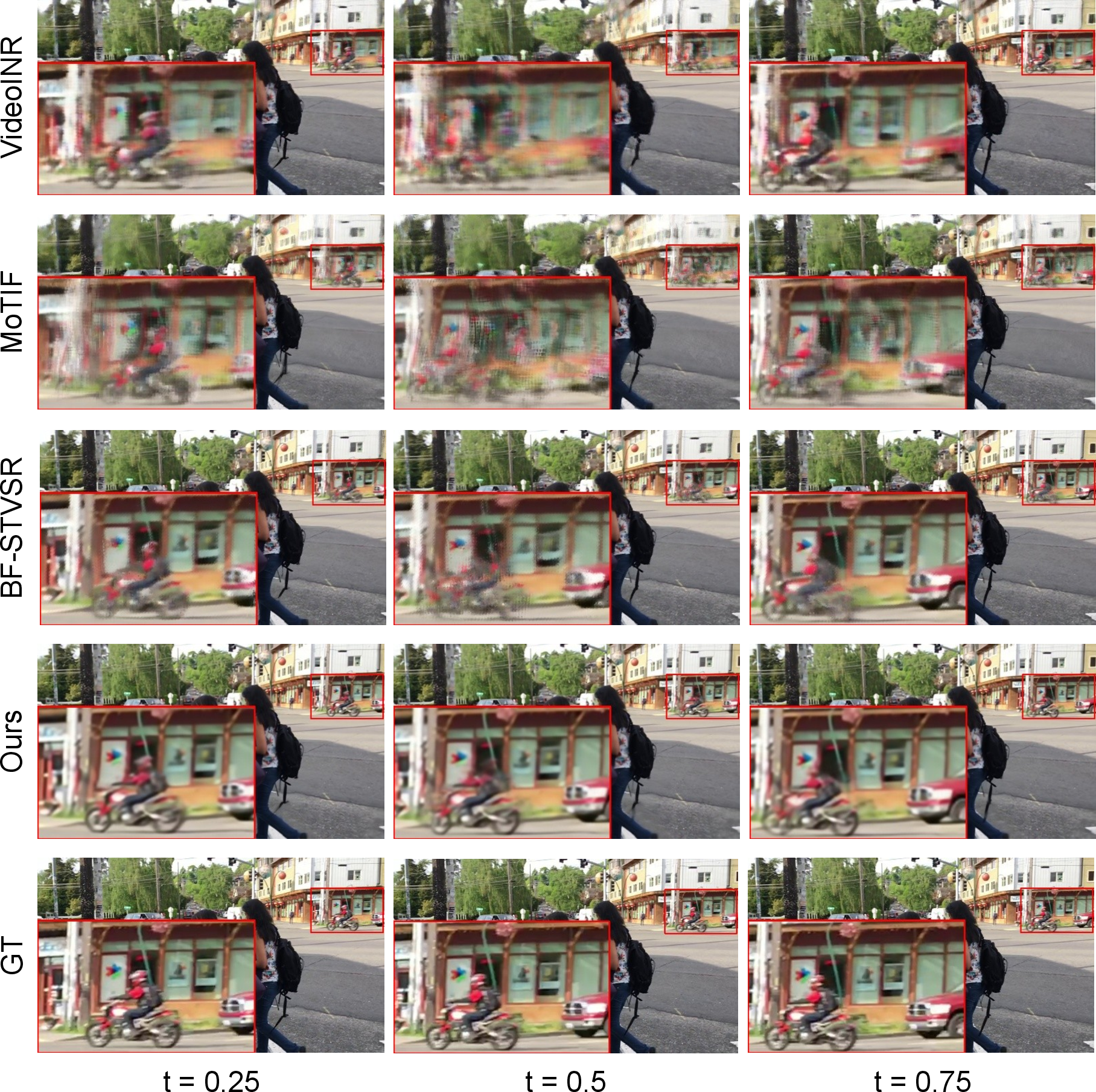
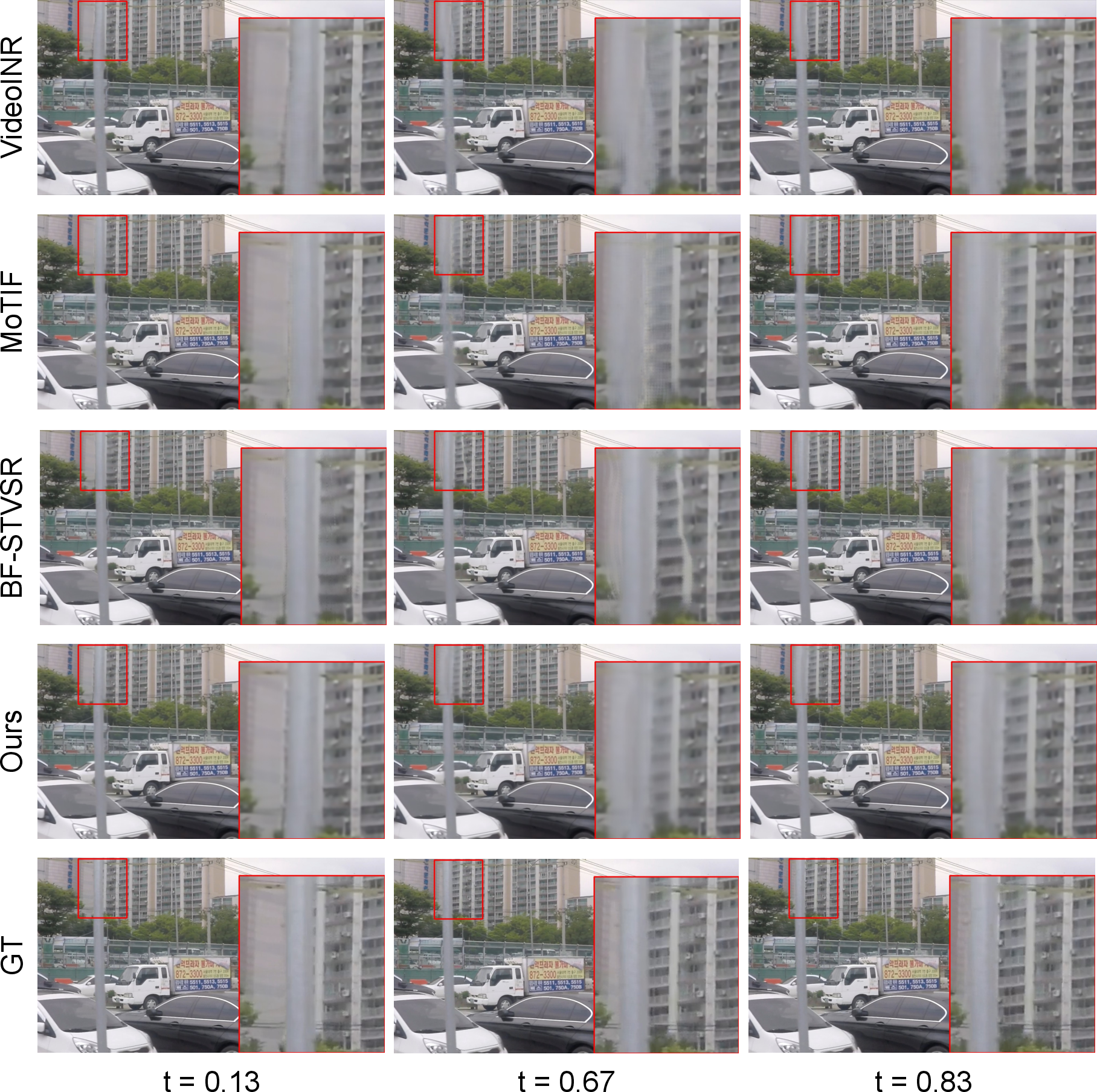
Figure 5: Qualitative comparisons of different C-STVSR methods on in-distribution time scale. The spatial scaling factor is set to x4 and the temporal factor to x8. Best viewed zoomed in.

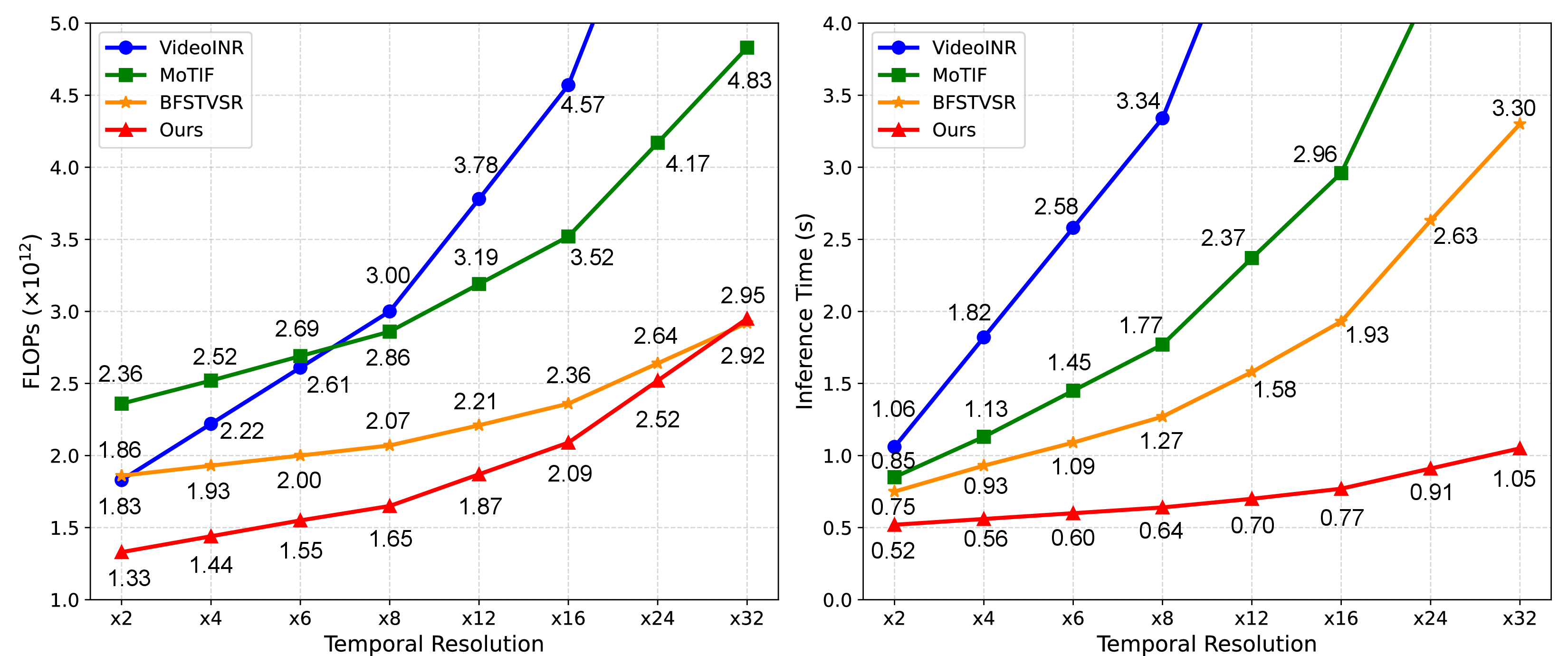
Figure 6: Computational cost (FLOPs, left) and inference time (right) comparison at $\Sigma_0, \Sigma_1$5 resolution with times 4 spatial upsampling across varying temporal scales (times 2--times 32).

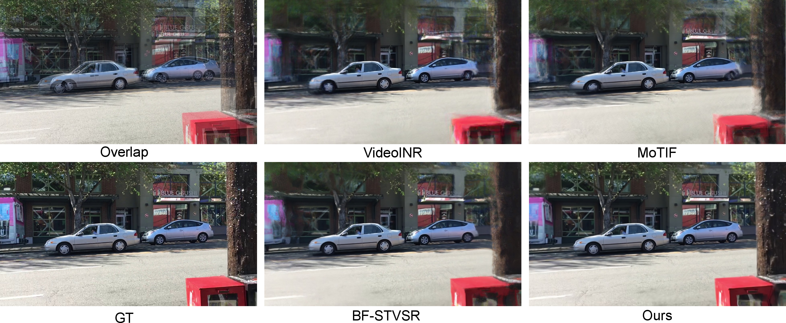
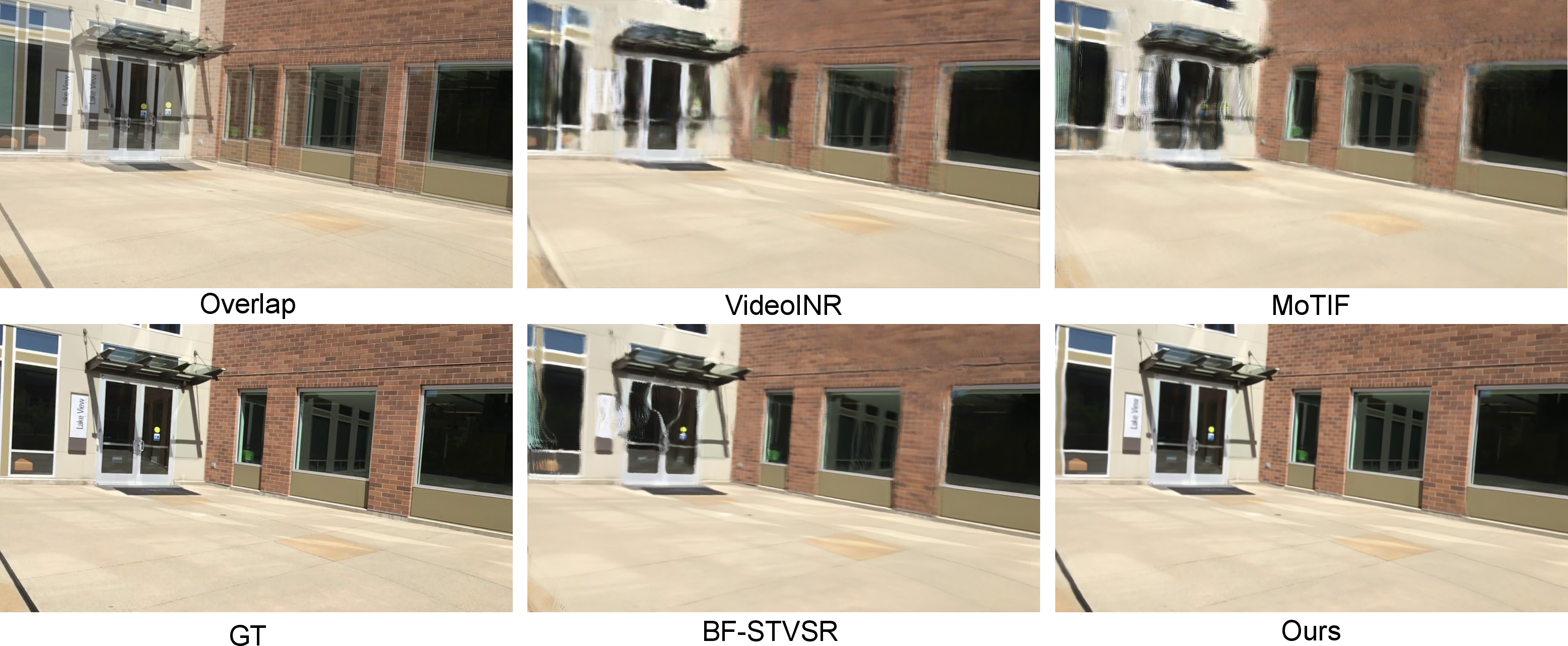
Figure 7: Qualitative comparison of different C-STVSR methods under large-scale global camera motions. (a) Visual results in a scenario with rapid camera zooming, where severe global scale changes occur. (b) Visual results under fast camera translation, causing massive global pixel shifts. Best viewed zoomed in.

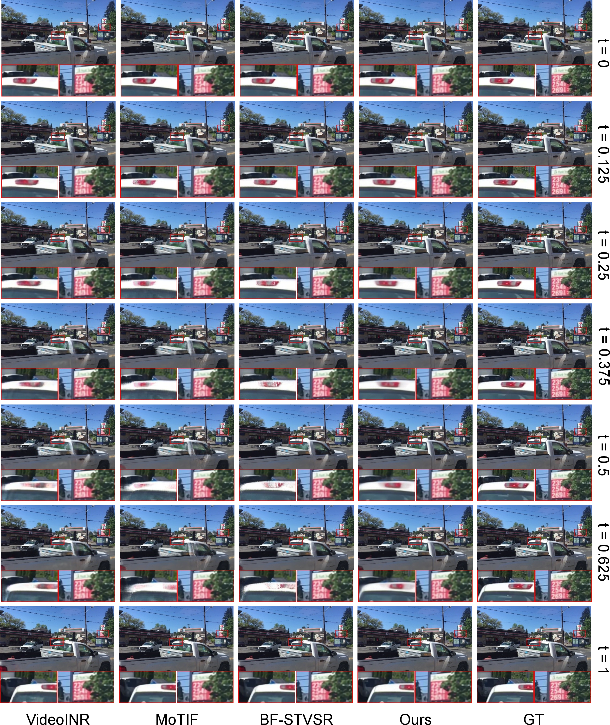
Figure 8: Qualitative comparisons of different C-STVSR methods on in-distribution time scale. The spatial scaling factor is set to times 4 and the temporal factor to times 8. Best viewed zoomed in.

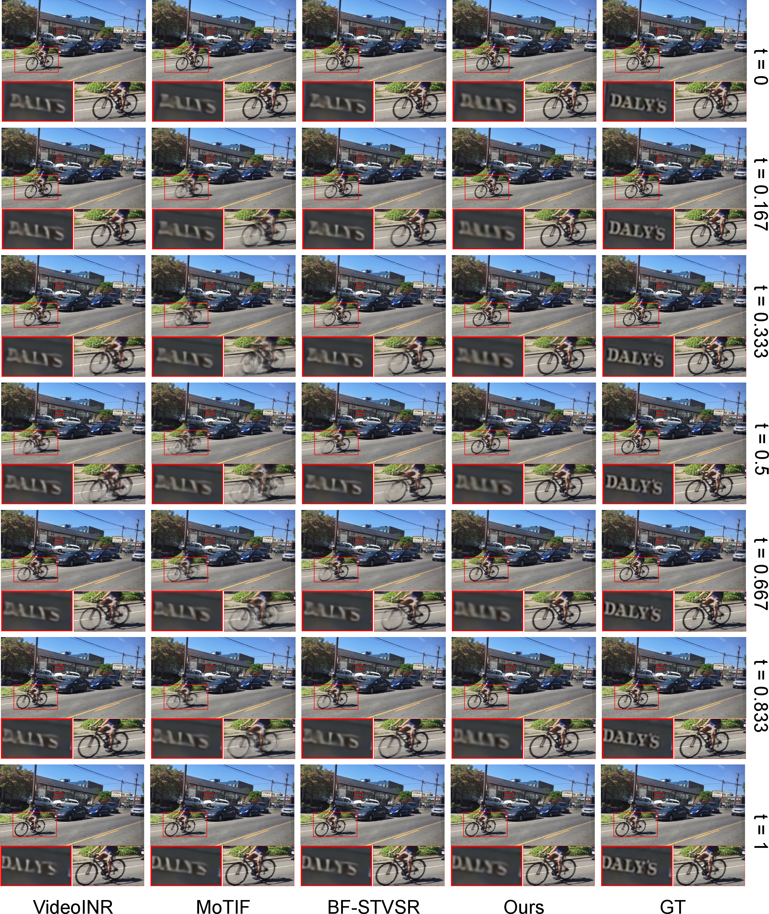
Figure 9: Qualitative comparisons of different C-STVSR methods on out-of-distribution time scale. The spatial scaling factor is set to times 4 and the temporal factor to times 6. Best viewed zoomed in.

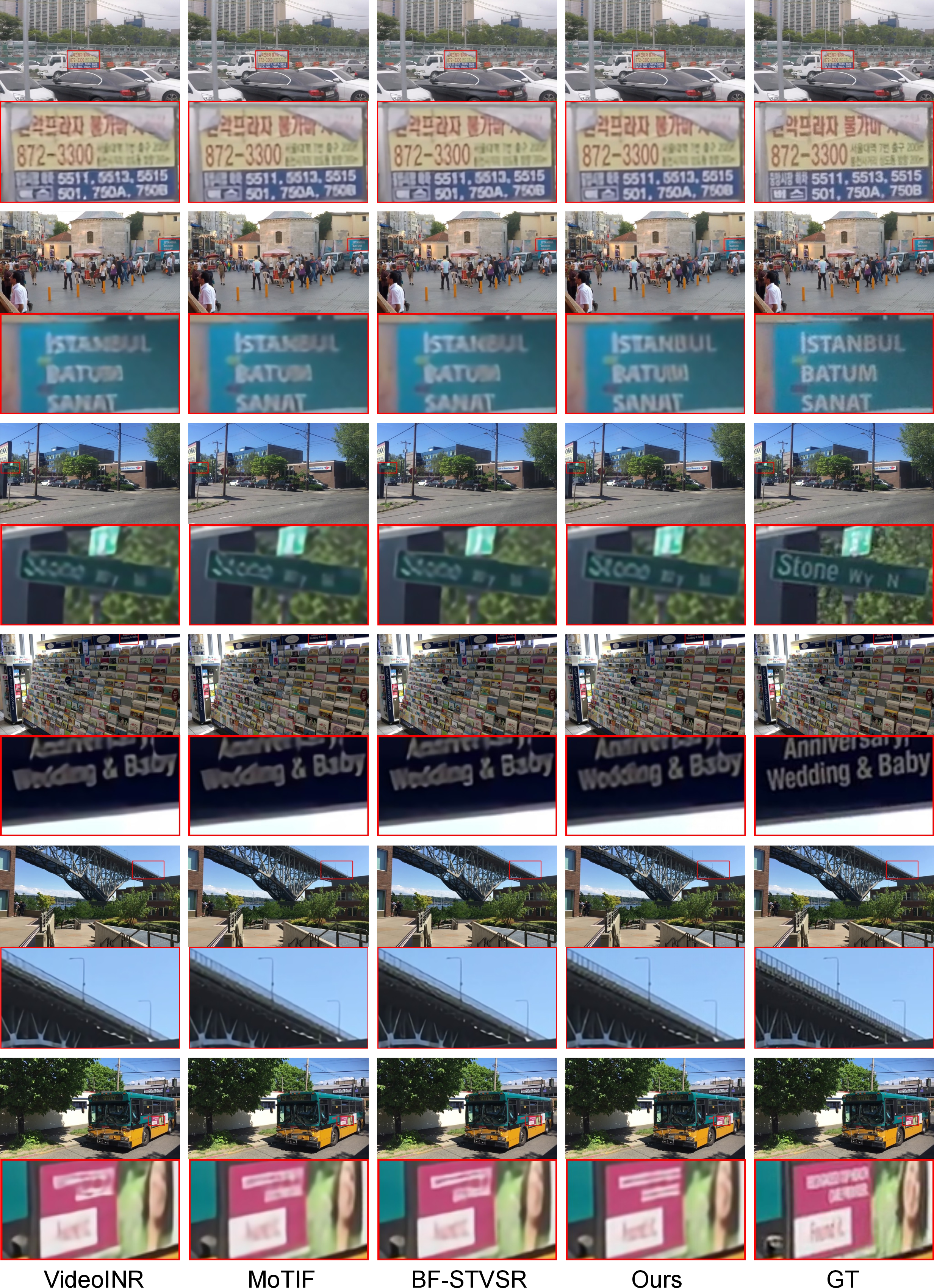
Figure 10: Qualitative comparison of different C-STVSR methods in the VSR task. The spatial scaling factor is set to times 4. Best viewed zoomed in.

Computational Efficiency

GS-STVSR demonstrates significant computational efficiency. Its inference time remains nearly constant at conventional temporal scales (×2–×8) and achieves over 3× speedup at extreme scales (×32) compared to BF-STVSR, with lower FLOPs (Figure 6). Specifically, when upscaling videos from 270p to 1080p with 8× temporal scaling, GS-STVSR achieves a pure rendering time of 0.4 seconds, more than 5 times faster than BF-STVSR, while using significantly less VRAM (15.5 GiB vs. 29.3 GiB). This efficiency is a direct consequence of the 2D-GS rendering mechanism, which bypasses the dense grid queries of INR-based methods, making it highly suitable for real-time video processing applications.

Ablation Study

Ablation studies confirm the efficacy of the proposed CRA and AOW modules. The full model, incorporating both, achieves the best performance. Removing either module or both results in a noticeable degradation. The removal of the CRA module, in particular, leads to training instability and performance drops, validating the importance of stable covariance prediction and drift prevention.

Implications and Future Work

The GS-STVSR framework presents substantial theoretical and practical implications. Theoretically, it establishes a novel paradigm for continuous spatio-temporal video super-resolution, demonstrating that 2D Gaussian Splatting can overcome the inherent limitations of INR-based methods concerning computational efficiency and scalability. The empirical finding of strong temporal stability in Gaussian covariance parameters informs a more efficient model design. Practically, the ultra-efficient inference and superior reconstruction quality open avenues for real-time, high-fidelity video enhancement in diverse applications, including streaming, virtual reality, and medical imaging.

Future research directions include addressing the limitations of the linear motion assumption for optical flow interpolation by exploring learned non-linear motion models. Furthermore, end-to-end joint optimization of optical flow and Gaussian parameters could mitigate errors from pre-trained flow extractors. Investigating scene-adaptive Covariance Prior Banks may further enhance representational capacity for more diverse video content.

Conclusion

GS-STVSR is the first framework to extend 2D Gaussian Splatting to C-STVSR, effectively bypassing the computational bottlenecks of INR-based approaches. By leveraging the temporal stability of Gaussian covariances, the framework employs an ultra-lightweight prediction module, coupled with optical flow guidance and adaptive offset windows, to ensure accurate Gaussian evolution under diverse motions. The Covariance Resampling Alignment module is instrumental in preventing covariance drift. Extensive experiments demonstrate that GS-STVSR achieves state-of-the-art reconstruction quality with fewer parameters and significantly improved inference speed, particularly at challenging spatio-temporal scales. This establishes Gaussian representations as an exceptionally efficient paradigm for video enhancement, poised to influence future developments in real-time continuous video super-resolution.