Measuring the rate of glitches in interferometric gravitational wave detectors with a hierarchical Bayesian model

Abstract: Ground-based gravitational wave detectors are now routinely surveying the dark Universe, finding hundreds of collisions between compact objects such as black holes and neutron stars. However, terrestrial non-Gaussian noise artefacts, commonly known as glitches, reduce the sensitivity to signals and can overlap signals, producing biased astrophysical inferences. We introduce a hierarchical Bayesian model to measure the glitch rate, which improves upon existing trigger-counting methods in its capacity to measure the rate down into the low signal-to-noise regime without contamination from the Gaussian noise background, provided the population is accurately modelled. The methodology builds on standard hierarchical inference, but includes several novel features, including hierarchical inference with quantile compression (HIQC), a generic approximation method for the hierarchical recycled likelihood, and a time-domain rate estimated by fitting basis functions. We validate the methodology using simulated data with injected glitches and then apply it to data from the fourth LIGO-Virgo-KAGRA observing run, demonstrating time-resolved inferences of the glitch rate over a 24 h period. The inferred glitch rate is consistent with estimates from trigger counts, but does not require an arbitrary threshold and provides a more fine-grained view of the temporal behaviour. Finally, we demonstrate how our individual-detector rate estimates can be transformed into a coincident glitch probability and utilise this to validate that the retracted gravitational-wave candidate GW230630_070659 is likely a pair of coincident glitches.

• The paper introduces a hierarchical Bayesian framework to estimate glitch rates without relying on fixed SNR thresholds.
• It employs quantile-based compression (HIQC) for computational efficiency while inferring both time-dependent and population-level glitch properties.
• The approach outperforms traditional counting methods by providing robust uncertainty quantification and improved detection reliability in gravitational-wave analysis.

Hierarchical Bayesian Modeling for Glitch Rate Inference in Gravitational-Wave Detectors

Introduction

The robust detection of gravitational-wave (GW) events with interferometric detectors such as LIGO, Virgo, and KAGRA is fundamentally limited by non-Gaussian, transient instrumental artifacts termed glitches. Accurately measuring the glitch rate and understanding its time- and population-dependence are critical both for improving GW detection pipelines and for robust astrophysical inference, particularly as these glitches can mimic or obscure genuine astrophysical events at the single-detector level. Conventional approaches rely on SNR-thresholded trigger counting—typically obtained via the Omicron pipeline—which introduces arbitrary thresholds, ineffective separation of weak glitches from the Gaussian noise floor, and limited population-level modeling.

This paper introduces a hierarchical Bayesian framework enabling threshold-free, statistically principled estimation of the glitch rate and, when desired, its population properties and temporal variations. The model's structure directly leverages the full non-thresholded strain data and employs a physically motivated parameterized glitch model. Key contributions include a hierarchical inference structure, quantile-based compression (HIQC) for computational efficiency, and extensions for modeling both glitch-population parameters and time-dependent rates.

Methodology

Limitations of Counting-Based Approaches

Standard glitch rate estimation in GW data analysis involves counting Omicron-derived triggers exceeding fixed SNR thresholds and interpreting these counts under a Poisson process assumption. The core challenge arises because the SNR distributions of glitches and noise triggers overlap in realistic detector conditions, as shown in (Figure 1).

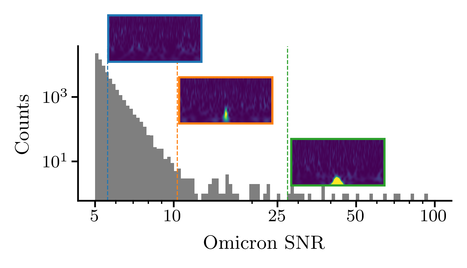
Figure 1: Histogram of Omicron trigger SNRs for a day of LIGO Livingston O4a data, with example time-frequency spectrograms at selected SNRs.

This ambiguity necessitates a delicate balance: lower thresholds introduce false positives from Gaussian noise, while higher thresholds yield underestimates by missing low-SNR glitches. Analysis of rate versus threshold (Figure 2) illustrates instability and sensitivity to threshold choice.

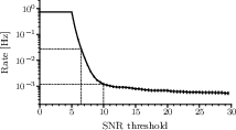
Figure 2: Estimated Poissonian glitch rate as a function of SNR threshold, highlighting the instability at low thresholds.

Hierarchical Bayesian Structure

The proposed methodology abandons thresholding by positing a generative model for glitches in the strain data and then deploying a two-level hierarchical Bayesian model:

• Level-I (segment-level): For each short data segment (chosen to be at most one glitch/segment), compute the evidence and posteriors for two models: a parameterized glitch model (antiglitch) and colored Gaussian noise.
• Level-II (population-level): Aggregate information from all segments under a mixture model, leveraging the Poissonian nature of glitches, and infer both the glitch rate and population-level hyperparameters.

For each segment, the key quantity is the Bayes factor (log-likelihood ratio) between the glitch and noise models. The approach admits seamless accommodation of time dependence (e.g., via spline basis for rate evolution) and population modeling (e.g., amplitude distributions). The structure of the hierarchical likelihood and its Bayes-optimal implementation allow for explicit marginalization and efficient likelihood reuse.

HIQC – Hierarchical Inference via Quantile Compression

Population-level inference rapidly becomes computationally burdensome for large datasets, due to the need for repeated evaluation of hyperlikelihoods over high-dimensional posterior samples. To address this, the HIQC approximation is introduced: decomposing event-level posteriors into quantiles, evaluating the likelihood only at quantile centers, and then aggregating with appropriate weights.

This is validated (Figure 3) to produce negligible bias with significant computational gain, scaling as O($N_{\mathrm{segments}} Q$) instead of O($N_{\mathrm{segments}} M$) where $Q \ll M$ (number of quantiles vs. number of posterior samples).

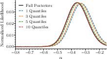
Figure 3: HIQC approximation validation—comparison of full vs. quantile-compressed likelihoods as quantile number varies.

Parametric Glitch Model

For Level-I inference, the antiglitch model—a frequency-domain analytic form characterized by central frequency, amplitude, bandwidth (precision), central time, and phase—is employed. This model is validated to give high likelihood for a wide variety of transient noise structures typical in single-interferometer GW data, although it intentionally targets short-duration glitches.

Validation on Simulations

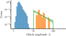
The hierarchical framework is validated by injecting well-characterized synthetic glitches, using generative modeling via normalizing flows trained on real detector glitch morphologies, into colored Gaussian noise.

Key findings:

• The hierarchical Bayesian method accurately recovers the true glitch rate and its credible intervals, matching the theoretical certainty for strong, separated (high SNR) glitches (Figure 4).
• As glitch SNR decreases and the amplitude distribution overlaps with that of noise, the hierarchical method remains unbiased only when the amplitude population distribution is simultaneously modeled. Omission of the correct population model (i.e., uniform/incorrect priors) yields significant rate underestimation for weakly separated cases (Figure 5).

  Figure 4: Log Bayes factor distribution for simulated glitches—vertical lines mark true glitch times.

  

  Figure 5: Noise-only vs. glitch amplitude distributions; power-law fit for simulated population.

• The hierarchical method returns robust, nonzero rate uncertainties even when the number of observed glitches is low (i.e., in the small-$n$ regime), outperforming pure counting estimators.

Application to Real LIGO Data

The method is deployed on a 24 hr segment of O4 LIGO Livingston data:

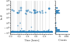
• Level-I analysis recovers Bayes factor time series consistent with Omicron triggers, although not all Omicron triggers correspond to large Bayes factors under the antiglitch model, primarily due to poor morphological compatibility (Figure 6).
• Posterior on the overall glitch rate (Figure 7), as well as its time-dependent spline-based version (Figure 8), are consistent with (and more fine-grained than) classical counting methods, with the rate following diurnal cycles likely tied to anthropogenic noise sources.

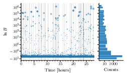
  Figure 6: Bayes factor time series for LIGO Livingston; right, its histogram.

  

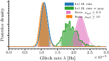
  Figure 7: Rate posterior from a full day’s Level-I analyses, compared to classical Omicron SNR-thresholded counting.

  

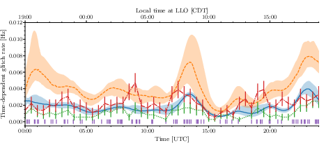
  Figure 8: Time-dependent inferred glitch rate; blue (glitch-only), orange (joint glitch and population). Hourly Poisson estimates (with Omicron SNR thresholds) included for comparison.

Computational Cost

While methodologically superior in terms of bias and modeling, the Bayesian approach is computationally expensive: Level-I inferences typically require 40 sec per 1 sec of data (Figure 9), due to the nested sampling used for evidence and posterior evaluation.

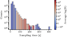
Figure 9: Histogram of Level-I segment compute times, colored by Bayes factor.

Coincident Glitch Probability Application

A critical practical application is the calculation of the probability of coincident glitches across detectors, relevant for interpreting marginal GW candidates. Taking GW230630_070659 as a test case, the method infers elevated individual glitch rates for both Hanford and Livingston during the candidate time.

Using the inferred Bayesian posterior on the rates, the method computes the probability that both detectors show an unrelated, but coincident, glitch within the inter-site light-travel window during a given timeframe—found to be substantial in this case (Figure 10), supporting the hypothesis that the event is terrestrial in origin.

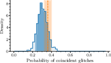
Figure 10: Posterior probability distribution for at least one pair of coincident glitches within an hour, estimated from the inferred rates and windows.

Discussion and Implications

Theoretical Impact

The presented hierarchical Bayesian framework transforms the estimation of glitch rates from an ad hoc, threshold-dependent counting exercise into a consistent, robust statistical inference problem. This enables:

• Unbiased estimation of glitch rates deep into the low-SNR regime.
• Joint inference of population model parameters (e.g., amplitude power-law exponents), essential for detector commissioning and characterization.
• Consistent uncertainty quantification even in the small-$n$ regime.

The model is modular: higher-level priors or additional glitch models can be trivially embedded via the mixture model formalism. Time-dependent rates and glitch sub-populations are directly supported, providing new avenues for GW detector noise characterization.

Practical Considerations

The major bottleneck is computational. Full Bayesian parameter estimation per segment (especially with MCMC/nested sampling) is currently expensive compared to Omicron's highly optimized pipeline. However, increasing computational resources and the emergence of ML-accelerated posterior inference schemes (e.g., simulation-based inference with normalizing flows [2025arXiv250812939D]) make scaling feasible.

The method is only as good as the adequacy of the glitch model—short glitches are well modeled, but low-frequency or long-duration transients may require an enriched basis or explicit multi-component modeling.

Future Directions

• Model enrichment: Incorporate additional glitch families and mixture likelihoods, potentially leveraging semi-supervised clustering tools such as those built on GravitySpy [2024EPJP..139..100Z].
• Population modeling: Extend to parameter spaces of greater dimension (e.g., joint amplitude, frequency, duration) and study time-dependence of population hyperparameters.
• Computational scalability: Adoption of gradient-based or amortized inference algorithms will make prospective "on-the-fly" glitch characterization feasible.
• Hybrid approaches: Integration with classical pipelines (Omicron) to triage and pre-select candidate glitch segments before expensive Bayesian modeling.

Conclusion

This work presents a comprehensive, statistically principled, and bias-free methodology for glitch rate inference in GW detectors. By eliminating the dependency on arbitrary SNR thresholds and directly modeling the population and time dependence, it opens the door to more accurate background modeling, improved search efficiency, and refined candidate classification—paving the way for more robust GW discovery and detector characterization.