A Dynamic Factor Model for Level and Volatility

Abstract: This paper develops a dynamic factor model in which common level and volatility factors evolve jointly, allowing conditional means and variances to interact endogenously within a large-information setting. The joint evolution of these factors provides a tractable framework for modeling risk, as fluctuations in volatility affect both the dispersion and the location of outcomes, generating state-dependent and asymmetric tail risks in predictive distributions. Volatility is captured by latent common factors that drive co-movement in second moments across a large panel, while heavy-tailed idiosyncratic shocks absorb transitory outliers and isolate persistent uncertainty dynamics. The framework embeds these interactions directly within a factor structure, allowing risk to arise endogenously from the joint dynamics of the system rather than being imposed through reduced-form approaches. Empirically, the model delivers systematic improvements in density forecast accuracy, particularly in the tails of the predictive distribution and at medium horizons. An application to international inflation highlights a dominant global level component in advanced economies and stronger regional and volatility contributions in emerging and developing economies, pointing to substantial heterogeneity in the role of uncertainty across countries.

• The paper introduces a unified dynamic factor model that embeds volatility-in-mean effects to capture state-dependent asymmetric tail risks.
• It employs a VAR structure with both level and volatility factors, estimated via Bayesian Gibbs sampling and particle methods.
• Monte Carlo and empirical applications demonstrate significant improvements in density forecast accuracy and robust tail risk assessment.

A Dynamic Factor Model for Level and Volatility

Introduction and Motivation

This paper introduces a large-dimensional dynamic factor model (DFM) that jointly models common level and volatility factors as endogenous state variables within a unified state-space system (2604.03681). The key contribution is the explicit VAR structure that allows for contemporaneous and lagged interactions between the factors governing the conditional means and volatilities of observed macroeconomic variables. By embedding volatility-in-mean effects directly into the factor model, the framework can capture state-dependent, asymmetric tail risk dynamics in predictive distributions—a feature central to Growth-at-Risk–type macroeconomic risk analysis.

This approach addresses known limitations of conventional large-information DFMs and VARs, which typically treat volatility as either exogenous or series-specific, thereby missing critical endogenous feedback between fluctuations in volatility and the conditional means of macroeconomic series. The modeling framework is motivated by persistent empirical evidence of systematic co-movement in volatility across macroeconomic panels and the increasing recognition that uncertainty shocks have effects on both the dispersion and the expected value of aggregate outcomes.

Model Specification and Estimation

The model generalizes the canonical large-dimensional DFM to jointly accommodate common level and volatility factors ($f_t, \mathcal{F}_t$), both evolving under a VAR process. Each observed series $X_{it}$ is expressed as

$X_{it} = B_i f_t + v_{it},$

where $B_i$ are factor loadings and $v_{it}$ are autocorrelated idiosyncratic components with conditional variance parameterized as

$$r_{it} = \exp(\mathcal{B}_i \mathcal{F}_t) \lambda_{it}^{-1},$$

allowing for heavy-tailed idiosyncratic components via a scale-mixture representation.

Crucially, the joint factor vector $F_t = [f_t^\top, \mathcal{F}_t^\top]^\top$ evolves according to a VAR($L$), with a general covariance matrix $\Omega$ capturing contemporaneous co-movement between level and volatility innovations. The model is estimated via Bayesian methods leveraging a Gibbs sampling scheme, with equation-by-equation posterior sampling of states, parameters, factor loadings, idiosyncratic shock scales, persistence parameters, and degrees-of-freedom for the heavy-tails. Particle Gibbs with ancestor sampling is utilized to address the nonlinearities in state evolution.

Monte Carlo Simulation and Identification

Monte Carlo experiments calibrating the DGP to the model specification confirm that the estimation procedure accurately recovers the dynamic paths of latent factors, cross-sectional factor loadings, autoregressive persistence parameters, and series-specific tail-thickness parameters across variables.

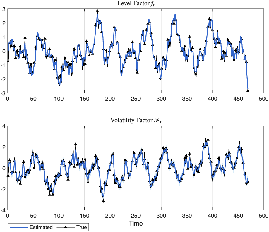
Figure 1: The estimated latent level and volatility factors closely track their true simulated counterparts over the sample, validating the identification and inference strategy.

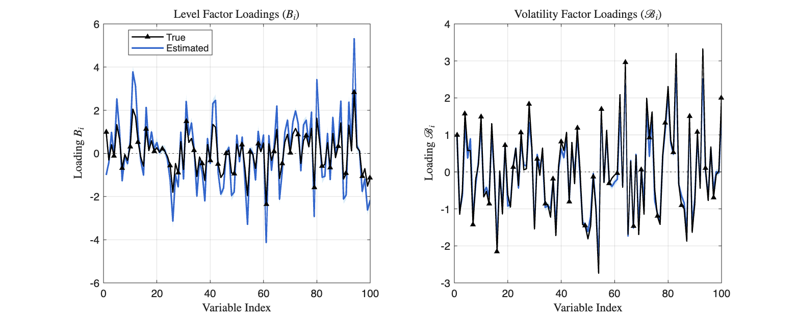
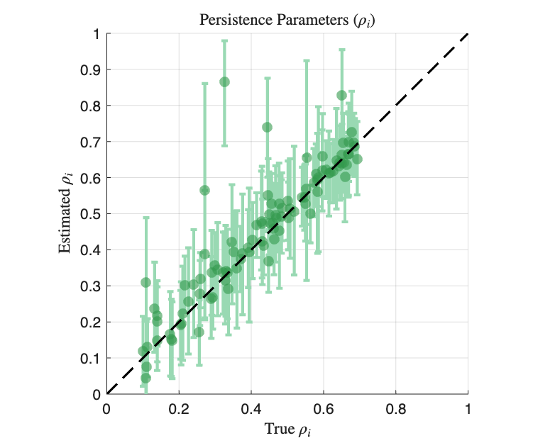
Figure 2: Cross-sectional scatter plots demonstrate that estimated level and volatility factor loadings reproduce their true values, indicative of robust identification across the panel.

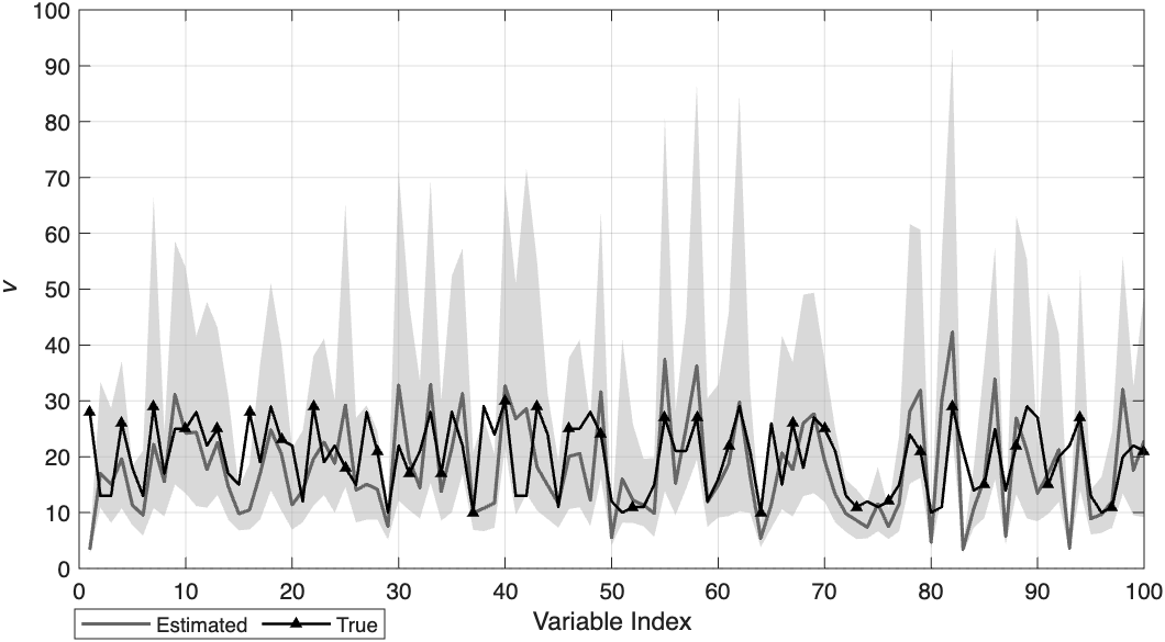
Figure 3: Estimated degrees-of-freedom for idiosyncratic Student-$t$ shocks align with their true, simulated values.

Empirical Application to U.S. Macroeconomic Panel

Applying the level–volatility DFM to a 105-variable U.S. macroeconomic panel (FRED-QD database) spanning more than six decades, the authors find that the dominant common volatility factor extracted from the panel is highly correlated with standard macroeconomic uncertainty indexes and spikes during the Global Financial Crisis and the COVID-19 period.

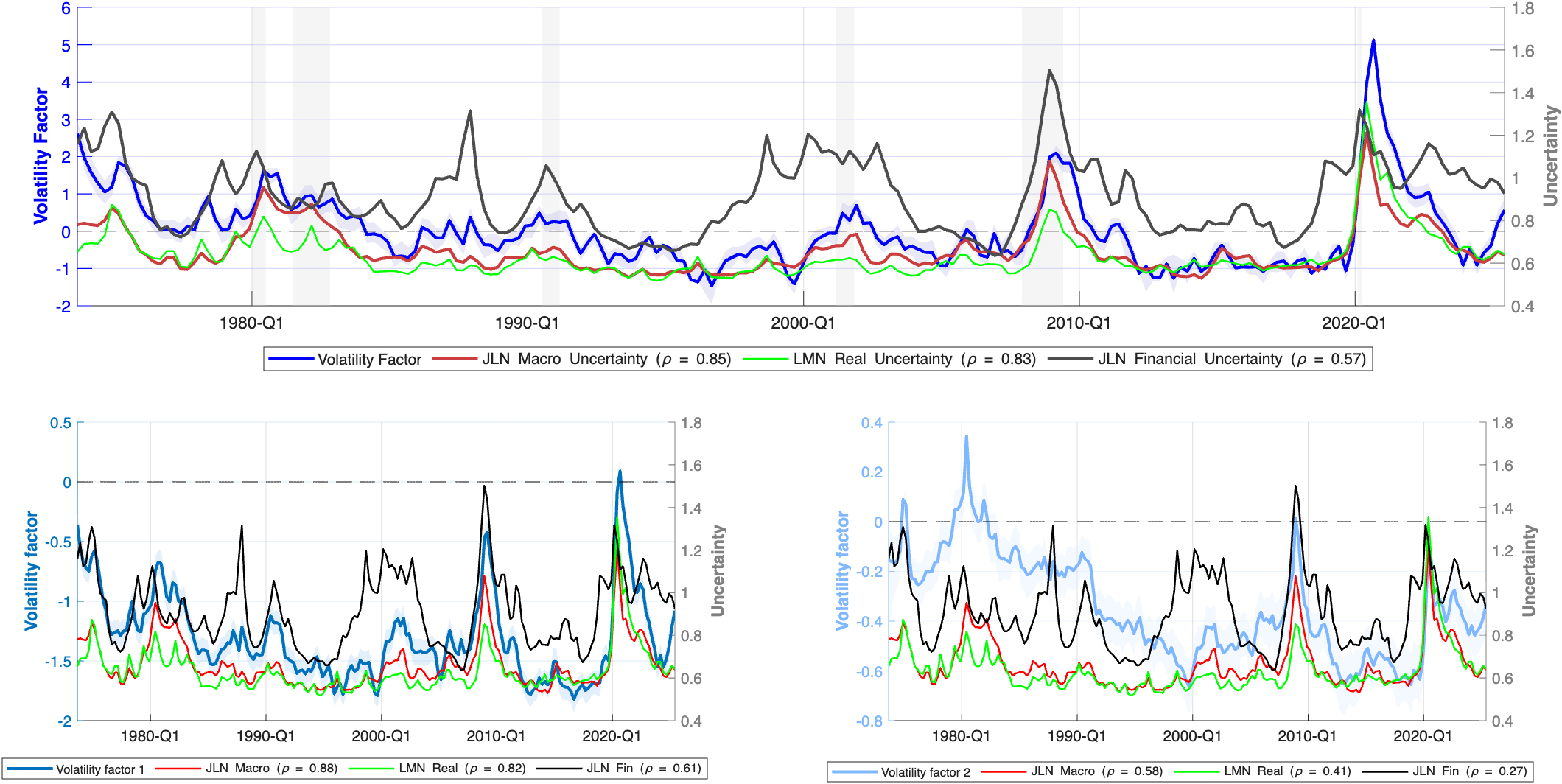
Figure 4: The estimated common volatility factors (one or two, depending on the specification) co-move strongly with external measures of macroeconomic uncertainty and exhibit pronounced episodes of volatility during stress events.

Predictive Density and Tail Risk Forecasting

Pseudo out-of-sample forecasting exercises reveal several pivotal results:

• Density forecast accuracy (measured by CRPS) is systematically and significantly improved when incorporating common volatility factors, especially in macro-labor and price variables and most notably in the distribution tails and at medium horizons.
• Point forecast accuracy (RMSE) remains virtually unaffected, indicating the model’s principal advantage arises in capturing risk, not central tendency.
• During high-volatility episodes, the interaction between level and volatility factors generates asymmetric tail dynamics, shifting and widening (especially the lower tail) of output and employment predictive densities and the upper tail of inflation.
• When benchmarked against quantile regressions targeting tail risk (i.e., Growth-at-Risk for output), the level–volatility DFM delivers competitive or superior threshold-weighted CRPS metrics, but within a coherent joint predictive density.

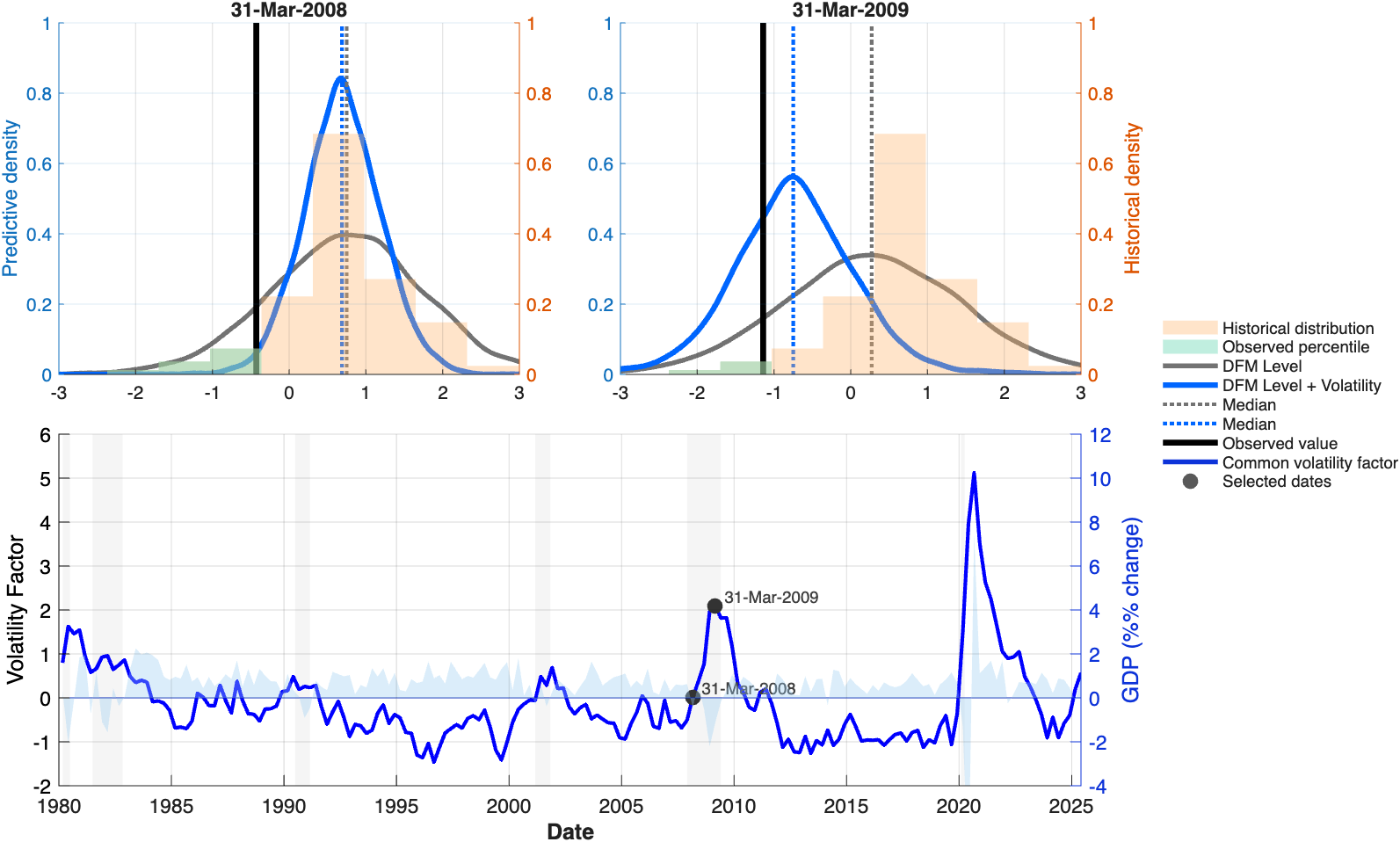
  Figure 5: Output growth predictive densities for GDP around the Global Financial Crisis illustrate how common volatility dynamically shifts the location and width of the one-step-ahead density.

  

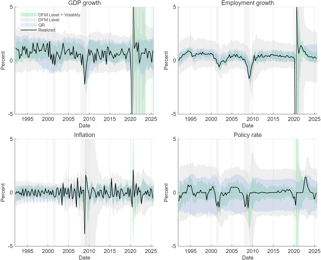
  Figure 6: Evolution of predictive quantiles for key variables, with the level–volatility DFM closely tracking realized extreme outcomes and outperforming standard DFMs and direct quantile regressions in tail sensitivity.

Numerical Evidence

CRPS-based loss ratios (relative to a benchmark DFM without common volatility factors) uniformly fall below unity for inflation, employment, and the funds rate, denoting strong improvements. Threshold-weighted CRPS (twCRPS) in the GDP lower tail and inflation upper tail are markedly better for the level–volatility DFM relative to both the DFM and (often) quantile regression benchmarks.

International Inflation Decomposition

A further empirical analysis decomposes inflation dynamics in a large panel of developed and emerging economies into global and regional factors for both levels and volatility. The results uncover:

• Advanced economies: Medium- and long-term inflation variance is dominated by a global level factor, with modest contributions from regional level and volatility factors.
• EMDEs: Marked heterogeneity is observed, with regional level and volatility factors often rivaling or exceeding the global factor’s influence, especially in Latin America and Sub-Saharan Africa.
• Volatility factors are particularly salient in EMDEs, evidencing heterogeneity in the source and propagation of inflation uncertainty.

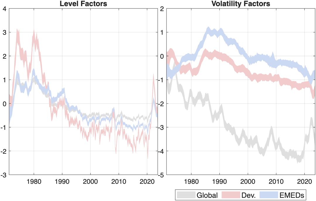
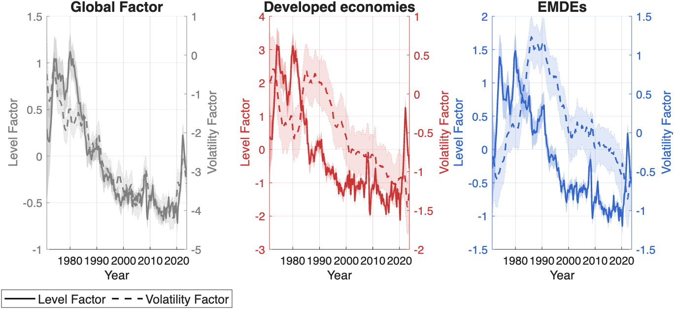
Figure 7: Joint dynamics of global and regional level and volatility factors driving international inflation across the sample.

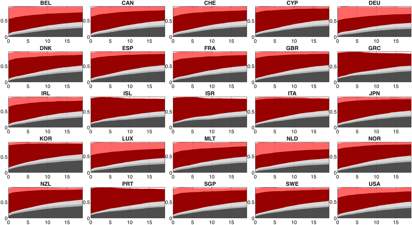
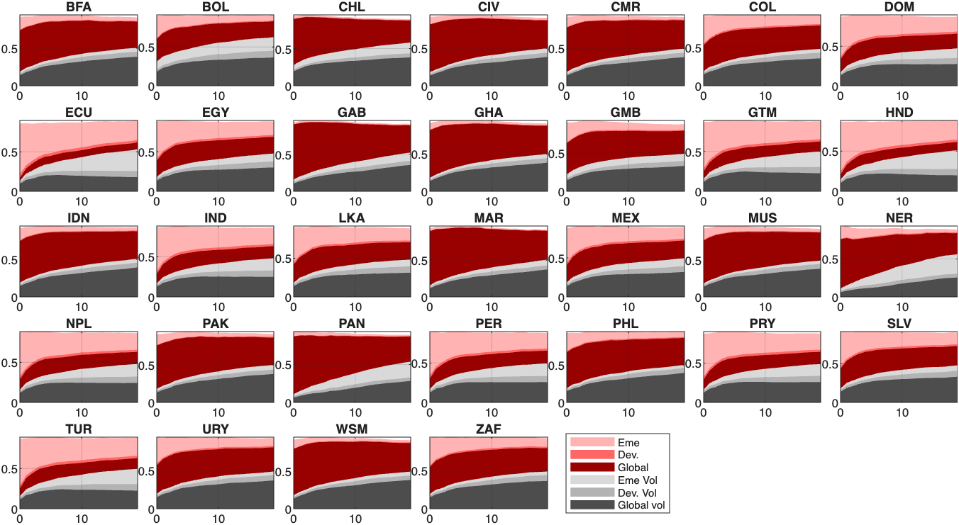
Figure 8: Country-level FEVDs for developed economies highlight the dominance of the global level factor in driving inflation variance.

Implications and Theoretical Significance

The VAR-based joint factorization of mean and volatility enables coherent, unified modeling of macro risk. The endogenous feedback between volatility and level factors captures time-varying risk asymmetries and tail behavior that are unaddressed by standard DFMs and exogenous volatility structures. Practically, these features yield large gains in real-time assessment of macroeconomic risk and inform more robust stress testing.

From a theoretical perspective, this work affirms that endogenous volatility-in-mean feedback is central for understanding macroeconomic risks in high-dimensional systems. It also provides a rigorous alternative to reduced-form quantile regression approaches, embedding the relevant tail risk dynamics within a generative, interpretable framework.

Further developments could extend this framework to incorporate nonlinear, non-Gaussian factor innovations, identification of shock sources, or upweighting of tail or regime-switching states.

Conclusion

The dynamic factor model for level and volatility factors delivers a unified, tractable, and empirically validated framework for capturing aggregate uncertainty, endogenous macro risk, and cross-sectional heterogeneity—especially in the tails of predictive distributions. The incorporation of common volatility factors as endogenous states moves beyond standard exogenous or series-specific volatility, generating robust improvements in density forecast accuracy and tail risk assessment, with critical implications for both cyclical macro monitoring and structural analysis of international inflation comovement and heterogeneity.