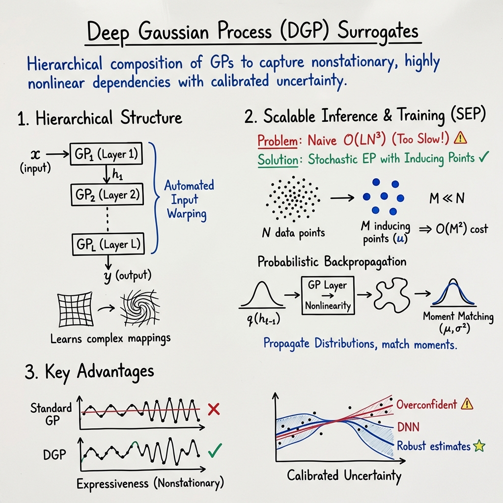
Deep Gaussian Process Surrogates

• Deep Gaussian Process surrogates are hierarchical models that compose multiple Gaussian process layers to capture nonlinear, nonstationary relationships in data.
• They utilize scalable inference techniques such as inducing points and stochastic expectation propagation to reduce computational cost while maintaining probabilistic accuracy.
• Probabilistic backpropagation enables recursive Gaussian moment matching, providing robust uncertainty quantification crucial for surrogate modeling in complex simulations.

Deep Gaussian Process (DGP) surrogates are a class of surrogate modeling techniques that generalize standard Gaussian processes through hierarchical (multi-layer) functional composition. Each layer in a DGP is a Gaussian process (GP), allowing input–output mappings to be recursively defined as compositions of GPs. This enables the surrogate to capture nonstationary, heteroscedastic, and highly nonlinear dependencies—properties frequently exhibited by complex computer experiments and scientific simulations. DGP surrogates are fully probabilistic, non-parametric, and offer superior capacity for modeling complex relationships and quantifying calibrated predictive uncertainty relative to shallow GPs or deterministic deep neural networks.

1. Hierarchical DGP Framework and Mathematical Structure

A DGP models the data-generating process as a composition of $L$ GP layers. For input $x$, the mapping proceeds as:

• Layer $\ell$ GP prior: $$p(f_\ell \mid \theta_\ell) = \mathcal{N\!GP}(f_\ell; 0, K_\ell)$$
• Hidden variable propagation:

$$p(h_\ell \mid f_\ell, h_{\ell-1}, \sigma_\ell^2) = \prod_n \mathcal{N}\big(h_{\ell,n}; f_\ell(h_{\ell-1,n}), \sigma_\ell^2\big)$$

with $h_{1,n} = x_n$ and final predicted output:

$$p(y \mid f_L, H_{L-1}, \sigma_L^2) = \prod_n \mathcal{N}\big(y_n; f_L(h_{L-1, n}), \sigma_L^2\big)$$

Unlike single-layer GPs, this stacked construction allows for automatic learning of input warping, dimensionality expansion or compression, and richer forms of kernel design, all in a data-driven, Bayesian manner. DGPs thereby model complex input–output relationships and uncertainty in high-dimensional, nonstationary settings (Bui et al., 2015).

2. Scalable Inference via Inducing Points and Stochastic Expectation Propagation

Naively, the cost of training a DGP is prohibitive, scaling as $O(LN^3)$ for $L$ layers and $N$ samples. To address this, sparse approximations using a set of inducing points $\mathbf{u}_\ell$ are employed at each GP layer, for example by the Fully Independent Training Conditional (FITC) method:

• Inducing prior: $$p(u_\ell \mid \theta_\ell) = \mathcal{N}(u_\ell; 0, K_{z_{\ell-1}, z_{\ell-1}})$$
• Layer transition: $$p(h_\ell \mid u_\ell, h_{\ell-1}, \sigma^2_\ell) = \prod_n \mathcal{N}(h_{\ell,n}; C_{n, \ell} u_\ell, R_{n, \ell})$$

This reduces per-layer training cost to $O(NM^2)$, with $M \ll N$ inducing points, and enables scalable model training.

Posterior inference in DGPs is analytically intractable, particularly with multiple layers and approximate conditionals. Stochastic Expectation Propagation (SEP) is adopted for scalable approximate Bayesian inference:

$q(u) \propto p(u)[g(u)]^N$

where $g(u)$ is a Gaussian “average” factor representing a typical data effect, decoupling the memory cost of inference from dataset size. SEP proceeds by sequentially forming cavity distributions, updating with single-likelihood “tilted” moments, and refining $g(u)$. This approach preserves analytic tractability of many updates and enables stochastic optimization with memory cost $O(M^2)$, independent of $N$ (Bui et al., 2015).

3. Probabilistic Backpropagation for Gaussian Moment Matching

A central step in learning and prediction is propagating distributions through the nonlinear hierarchy of GPs. This is most tractable for Gaussians, but deep compositions generally result in non-Gaussian outputs. Probabilistic backpropagation addresses this by, at each layer, matching moments (mean and variance) of the output to a Gaussian, enabling recursive, approximate inference:

• Cavity update: $$q^{\setminus 1}(u) = \mathcal{N}(u; m^{\setminus 1}, V^{\setminus 1})$$
• Posterior update (for one datapoint, after moment matching):

$$m = m^{\setminus 1} + V^{\setminus 1} \nabla_{m^{\setminus 1}} \log \mathcal{Z}$$

$$V = V^{\setminus 1} - V^{\setminus 1}\left[\nabla_{m^{\setminus 1}} \log \mathcal{Z}\left(\nabla_{m^{\setminus 1}}\log\mathcal{Z}\right)^\top -2\nabla_{V^{\setminus 1}}\log\mathcal{Z}\right] V^{\setminus 1}$$

where $\mathcal{Z}$ is the data likelihood “normalization” under the current approximation, recursively computed via Gaussian marginalization at each DGP layer (Bui et al., 2015).

In two-layer DGPs, integrals such as

$$\mathcal{Z} = \iint dh_1 du_2 \, p(y|h_1,u_2)q^{\setminus 1}(u_2) \int du_1 p(h_1|x,u_1)q^{\setminus 1}(u_1)$$

are approximated by successive moment matching, using analytic forms for kernels like the exponentiated quadratic under Gaussian input. This makes DGP moment propagation computationally efficient.

4. Advantages in Representational Power and Uncertainty Quantification

DGP surrogates present several key advantages over standard GPs:

• Automated Adaptive Warping: DGPs adaptively re-map the input space, discovering nonlinear transformations appropriate for the data, thereby constructing sophisticated data-driven kernels.
• Expressiveness: The multi-layer structure captures nonstationary and higher-order interactions unreachable by single-layer models.
• Well-Calibrated Uncertainty: Hierarchical composition provides refined uncertainty estimation. By propagating predictive covariance through layers, uncertainty is sensitive to latent representations and modelled function complexity.
• Scalability: Inducing point methods and SEP-based inference enable DGP surrogates to scale to substantial real-world datasets.
• Empirical Performance: On benchmark datasets such as Boston Housing, DGPs trained with SEP and probabilistic backpropagation outperform traditional GP regression in RMSE and mean log loss, and are never worse than state-of-the-art alternatives (Bui et al., 2015).

5. Practical Considerations and Limitations

• Computation: DGPs require more computation than shallow GPs, but SEP reduces memory overhead from $O(NM^2)$ (full EP) to $O(M^2)$. Using minibatch stochastic optimization (e.g., Adam) is essential for large data.
• Inducing Point Placement: Performance benefits from well-placed inducing inputs. Approximations can introduce “approximation repair” effects in DGPs, as higher layers are able to compensate for induced errors at lower layers.
• Approximation Error: Moment matching introduces bias in non-Gaussian regimes, but effectiveness is sustained in practical datasets using analytic moment propagation for common kernels.
• Depth: Empirically, two or three layers often suffice; deeper structures can be more difficult to train reliably.

6. Applications, Impact, and Related Developments

DGP surrogates are widely applicable where flexibility, nonstationarity, and robust uncertainty quantification are crucial. Examples include:

• Scientific and Engineering Simulations: Surrogate modeling of computationally intensive simulators with complex, non-stationary response surfaces.
• Automated Bayesian Kernel Design: Data-driven learning of warping and expansion/compression avoids manual feature engineering.
• Active Learning and Bayesian Optimization: DGP uncertainty quantification informs acquisition strategies in sequential experimental design settings.

Related advancements leverage DGP frameworks in diverse inferential settings—for instance, Bayesian inverse problems, active learning with complex simulators, and multi-task modeling—due to their capacity for both flexible function approximation and rigorous uncertainty modeling (Bui et al., 2015).

---

In summary, Deep Gaussian Process surrogates, as realized through sparse inducing point approximations, stochastic expectation propagation, and probabilistic backpropagation, offer a tractable, scalable Bayesian surrogate modeling solution that flexibly adapts to complex, non-stationary relationships and provides high-quality uncertainty estimates, outperforming conventional Gaussian Process regression across benchmark tasks.