Hedging market risk and uncertainty via a robust portfolio approach
Abstract: Shorting for hedging exposes to risk when the market dynamics is uncertain. Managing uncertainty and risk exposure is key in portfolio management practice. This paper develops a robust framework for dynamic minimum-variance hedging that explicitly accounts for forecast uncertainty in volatility estimation to achieve empirical stability and reduced turnover, further improving other standard performance metrics. The approach combines high-frequency realized variance and covariance measures, autoregressive models for multi-step volatility forecasting, and a box-uncertainty robust optimization scheme. We derive a closed-form solution for the robust hedge ratio, which adjusts the standard minimum-variance hedge by incorporating variance forecast uncertainty. Using a diversified sample of equity, bond, and commodity ETFs over 2016-2024, we show that robust hedge ratios are more stable and entail lower turnover than standard dynamic hedges. While overall variance reduction is comparable, the robust approach improves downside protection and risk-adjusted performance, particularly when transaction costs are considered. Bootstrap evidence supports the statistical significance of these gains.

Paper Prompts
Sign up for free to create and run prompts on this paper using GPT-5.
Top Community Prompts
Explain it Like I'm 14
Hedging market risk and uncertainty via a robust portfolio approach — explained simply
What this paper is about
This paper looks at a safer way to hedge investments. Hedging means using another, related asset to offset (protect against) losses. The authors focus on how to choose the “hedge ratio,” which tells you how much of the hedging asset to use. Their main idea is to build hedge ratios that stay steady and work well even when market forecasts are uncertain, so investors don’t have to trade too often or pay too many fees.
What questions the paper asks
The authors set out to answer a few practical questions:
- Can we build hedge ratios that don’t jump around a lot day to day?
- Can we make hedges that still reduce risk when the future is uncertain or noisy?
- Do these more “robust” hedges perform better once you include real-world costs like trading fees?
- Does this work across different types of assets (stocks, bonds, commodities) and across different market conditions?
How the researchers approached the problem
Think of this like planning for a rainy day:
- If you only trust a single precise weather forecast, you might get soaked if it’s wrong.
- If you plan for a range of possible weather (sunny to rainy), you’ll carry an umbrella when it’s most sensible.
The paper does something similar with financial risk:
- Using better measurements of daily risk
- They measure daily volatility (how much prices move) using many short intraday price changes (like checking the weather every 5 minutes instead of once a day). This is called “realized volatility/covariance” and gives a clearer picture than just using daily closing prices.
- Forecasting the near future in a simple, explainable way
- They forecast future volatility using an autoregressive (AR) model. In simple terms: “tomorrow’s risk tends to be like a weighted average of recent days’ risk, plus some noise.” It’s like saying: if the last few days were stormy, tomorrow is also likely to be stormy.
- Planning for uncertainty with a safety margin
- Forecasts are never perfect. So instead of using just one forecast, they assume risk could be within a range (a “box” of possibilities). This is called a “box-uncertainty” set.
- They then choose the hedge ratio to perform well even in the worst-case within that range. This is called a “robust” hedge.
- A simple formula you can actually use
- The standard minimum-variance hedge ratio is roughly: h = covariance(S, F) / variance(F), where S is the asset you hold and F is the asset you short to hedge.
- The robust version the authors derive increases the denominator by a “buffer” that reflects the uncertainty in the forecasted variance of the hedging asset F. In plain words: when you’re less sure about risk, you hedge a little more carefully to avoid overreacting.
- Testing in the real world
- They test on a basket of ETFs from 2016–2024, including stocks (like S&P 500), bonds, and commodities (like oil and gold).
- They compare the robust hedge to the usual dynamic hedge across multiple time horizons (like daily vs. multi-day adjustments).
- They measure:
- Hedge effectiveness (how much risk is reduced)
- Downside protection (how well the hedge works when markets are falling)
- Turnover (how often you have to trade)
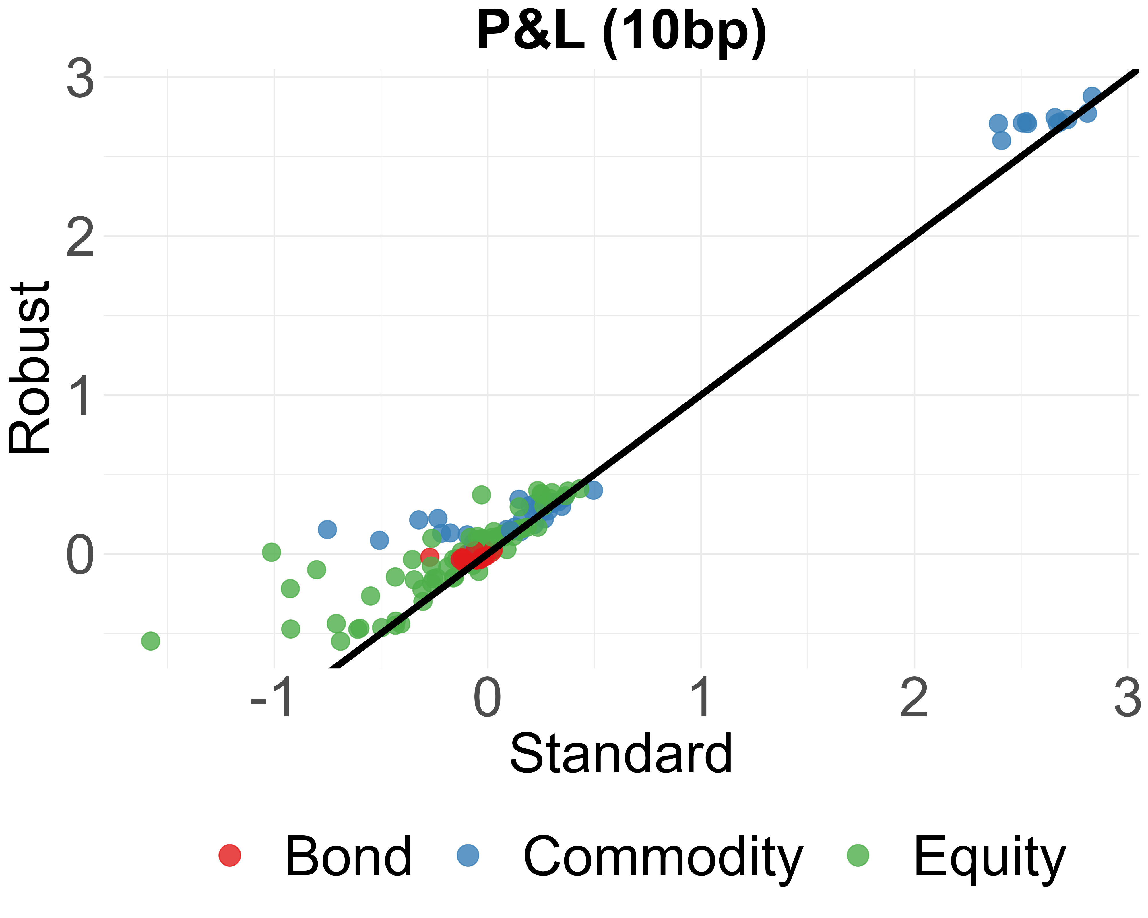
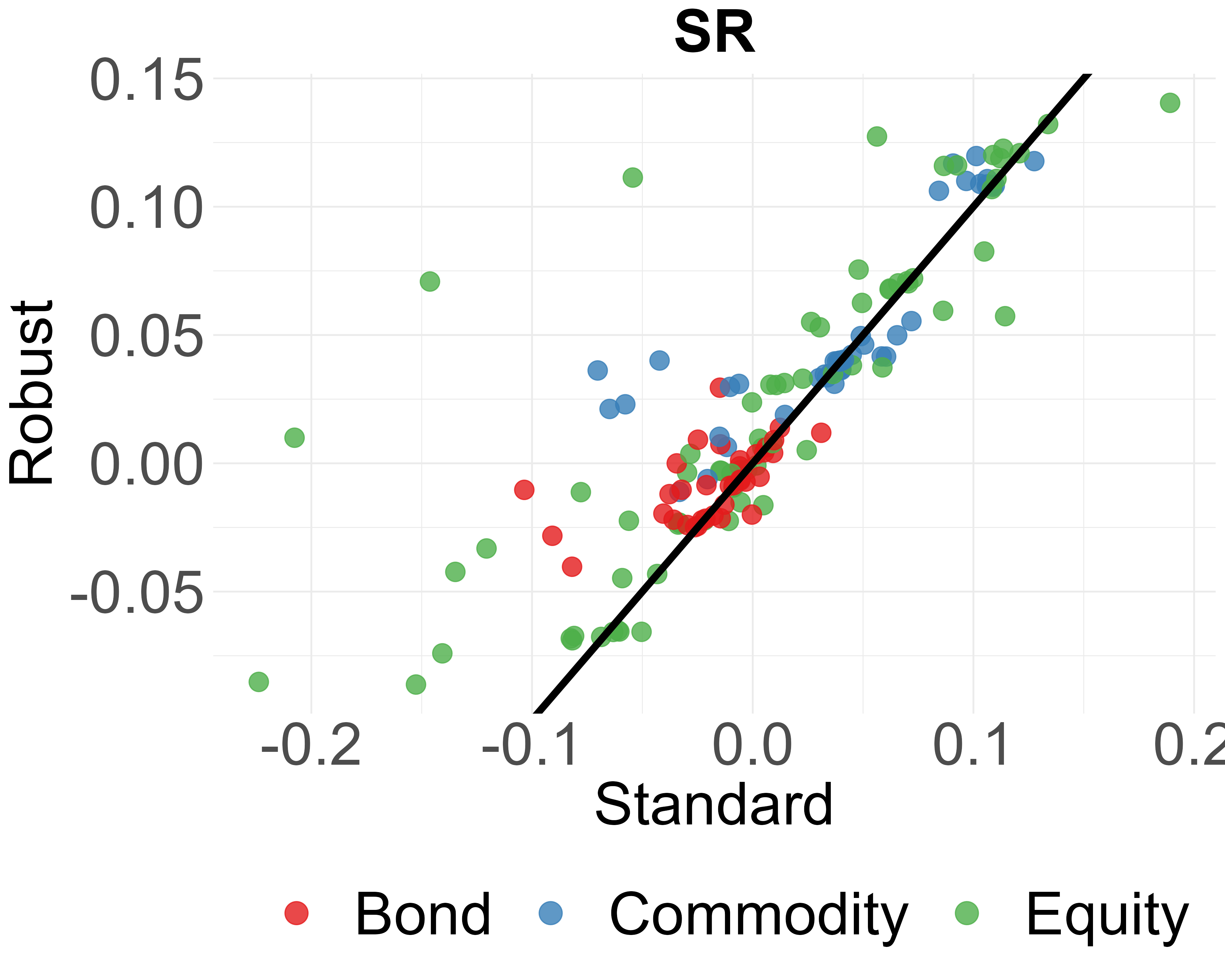
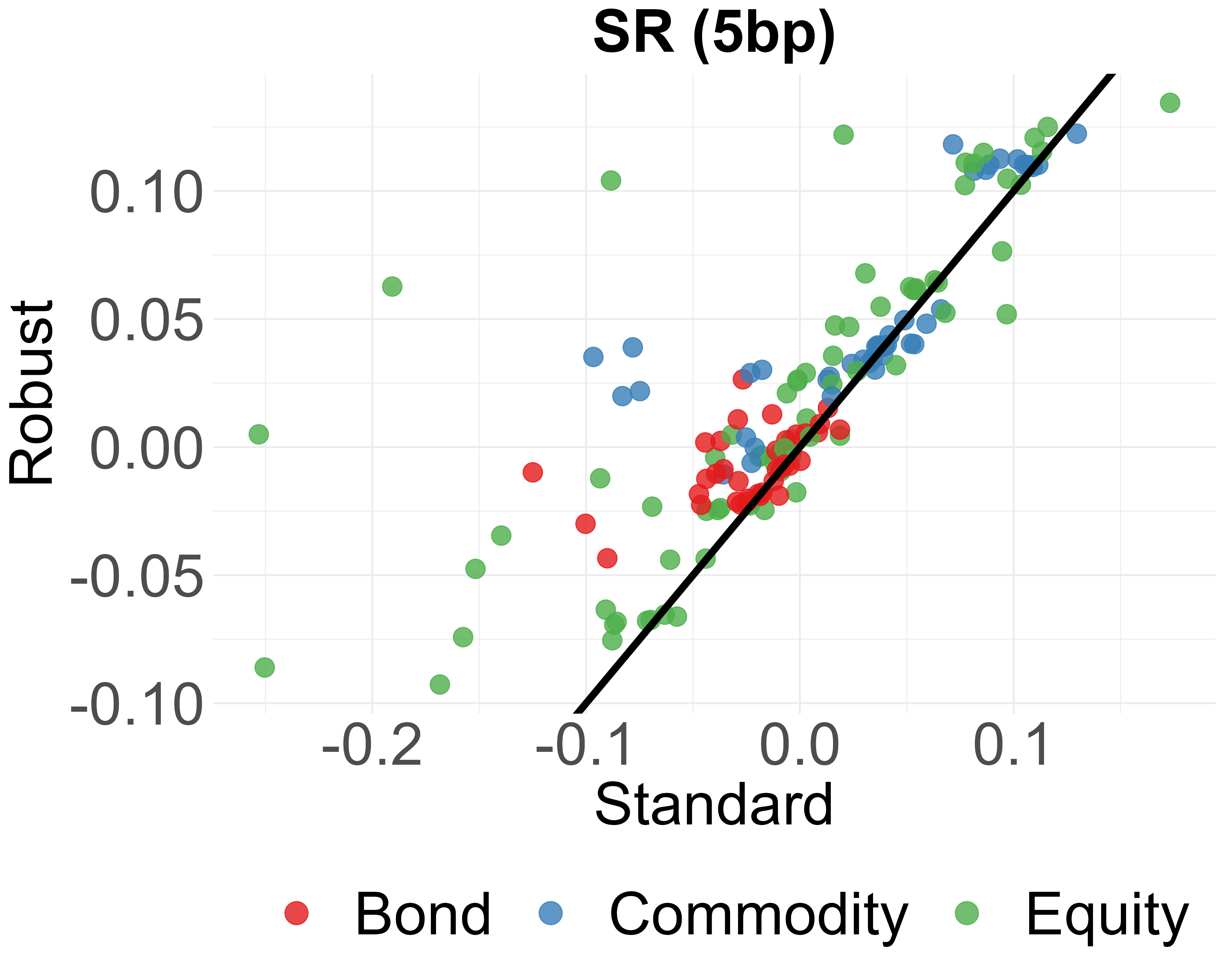
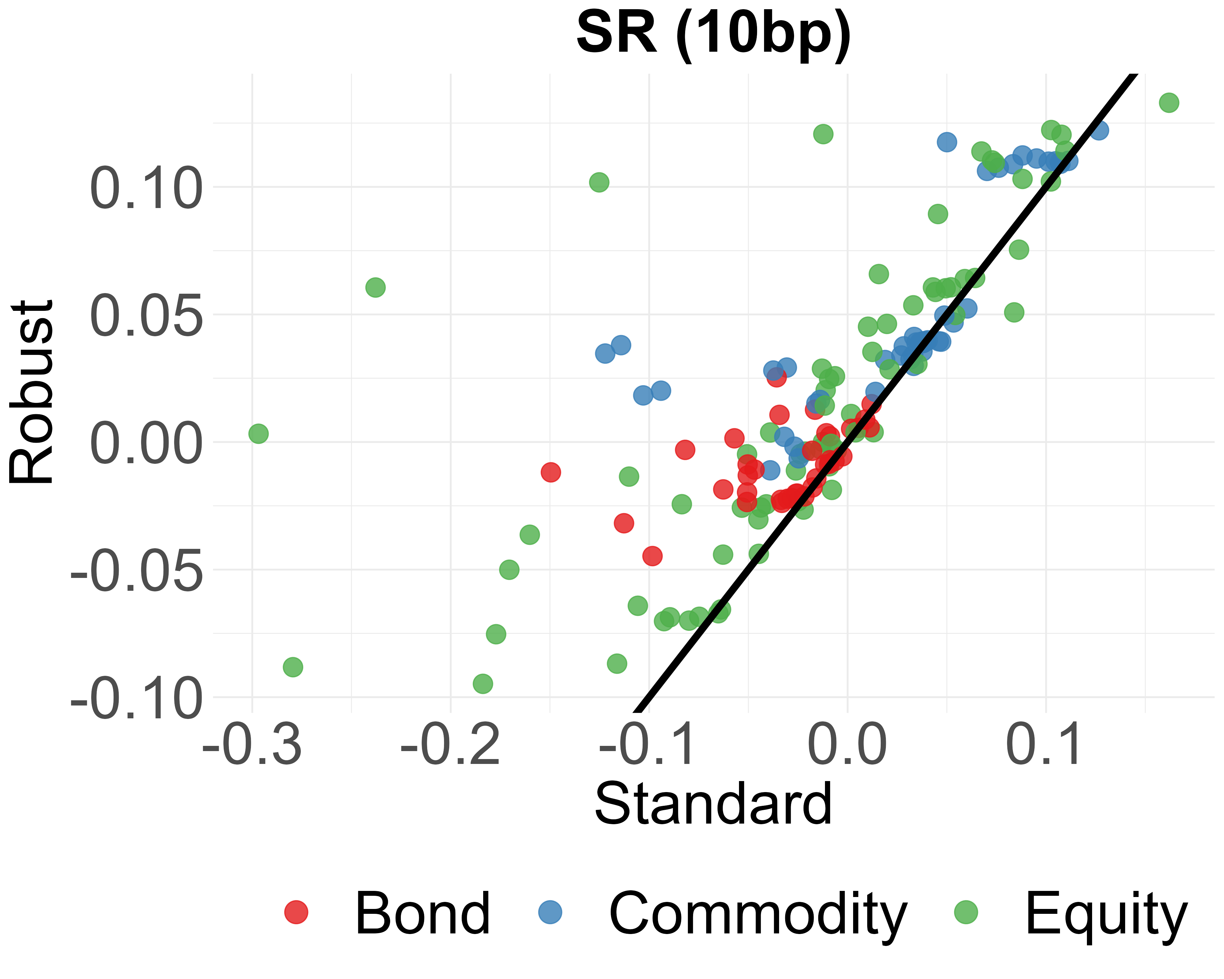
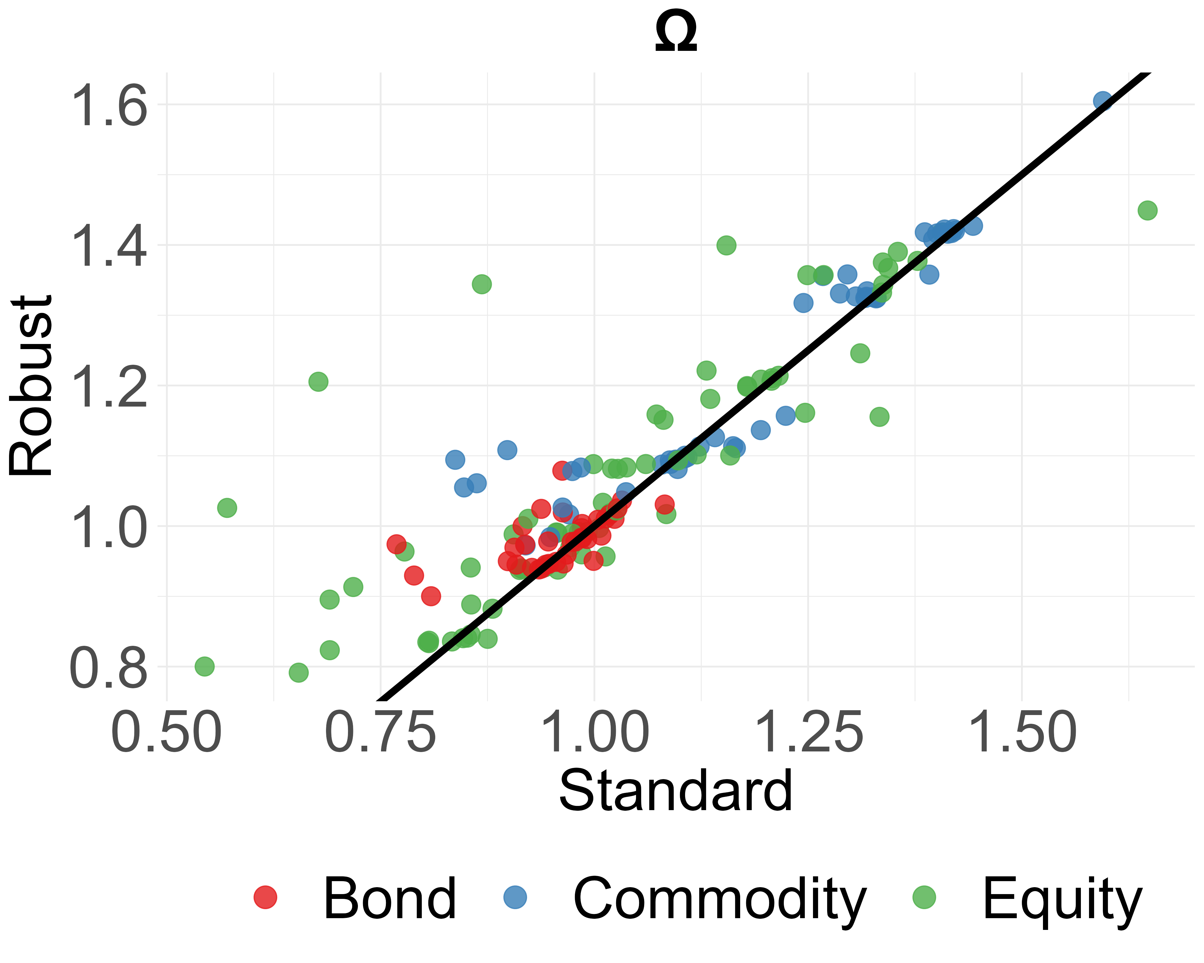
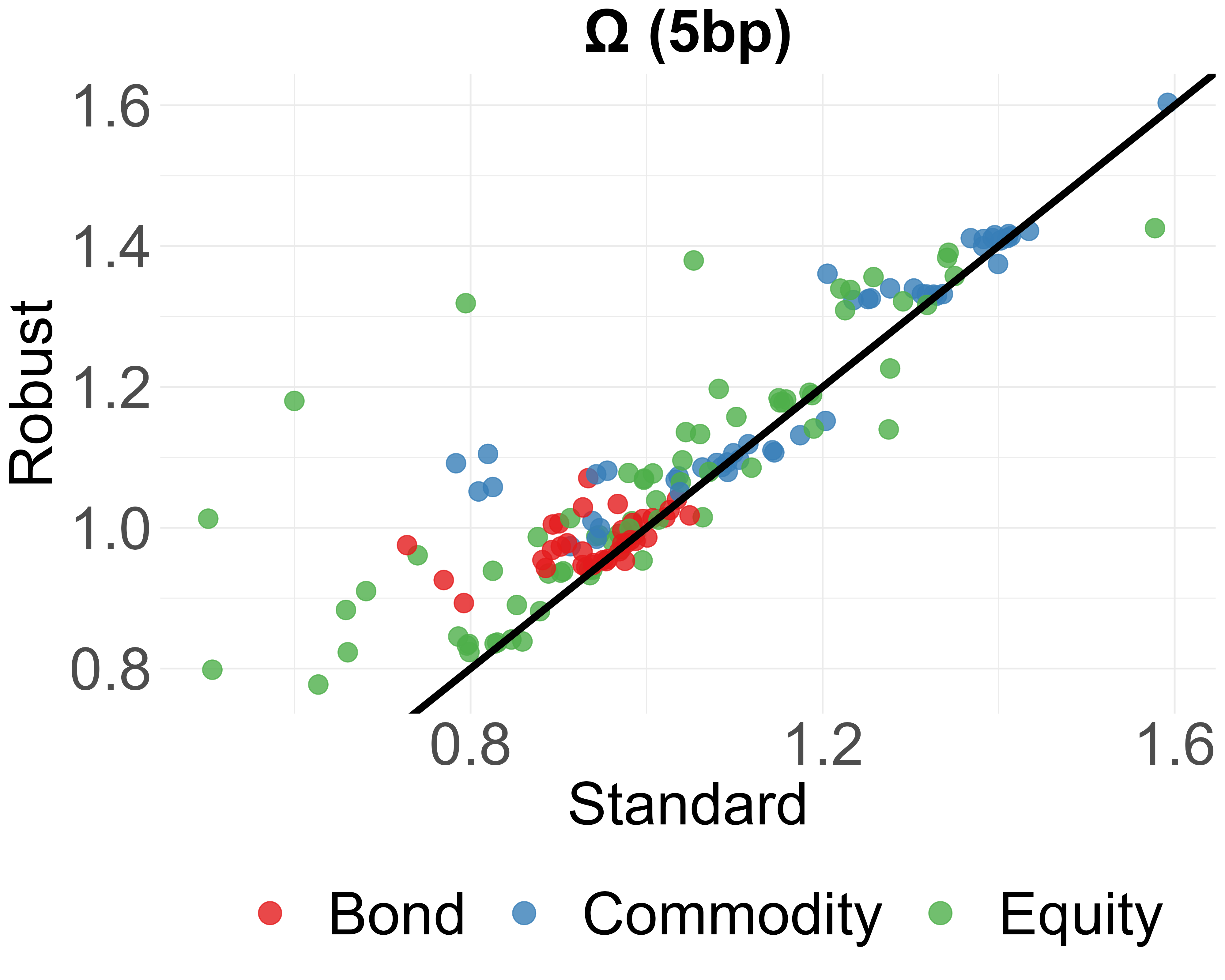
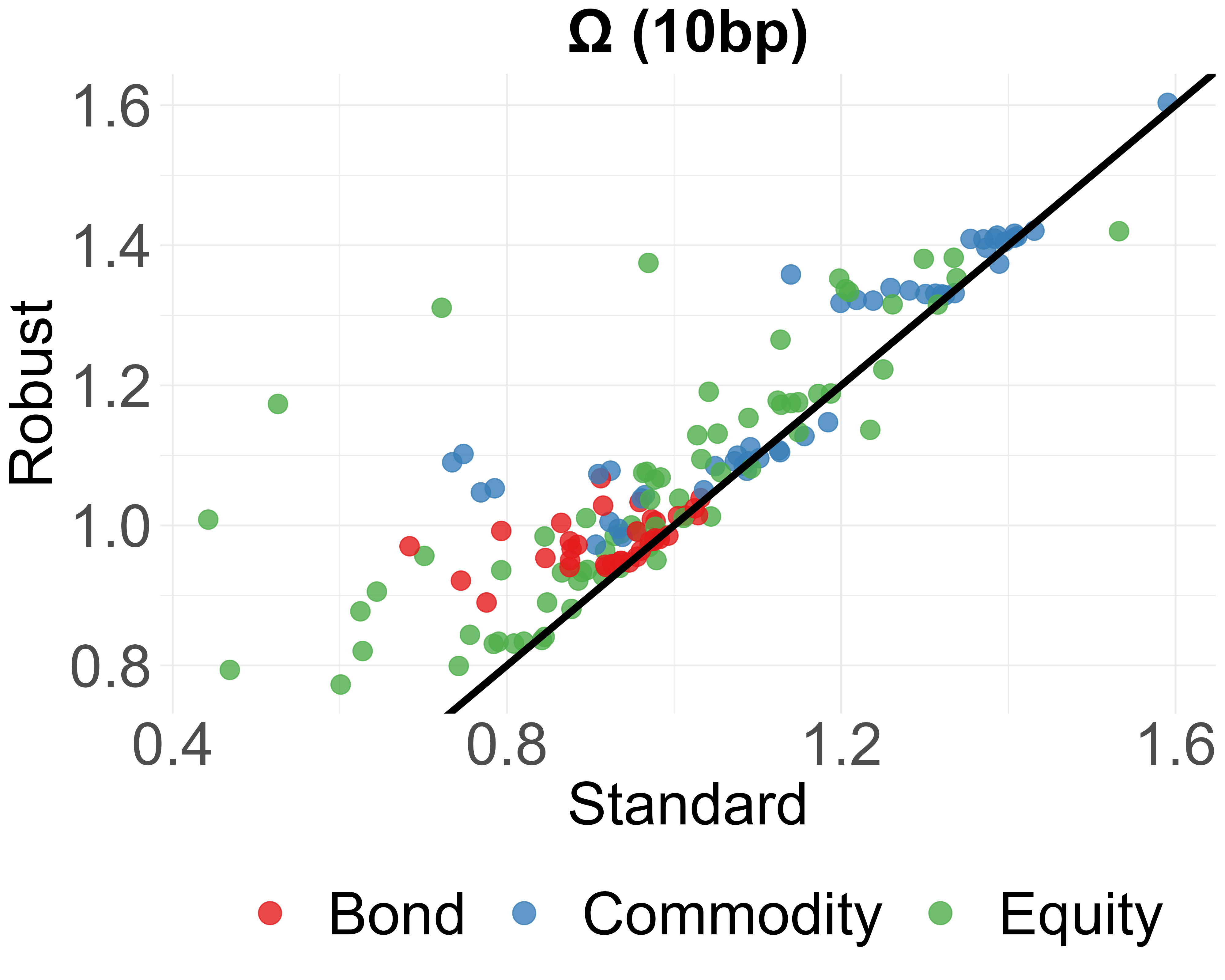
- Performance after costs (profit and loss, Sharpe ratio, Omega ratio)
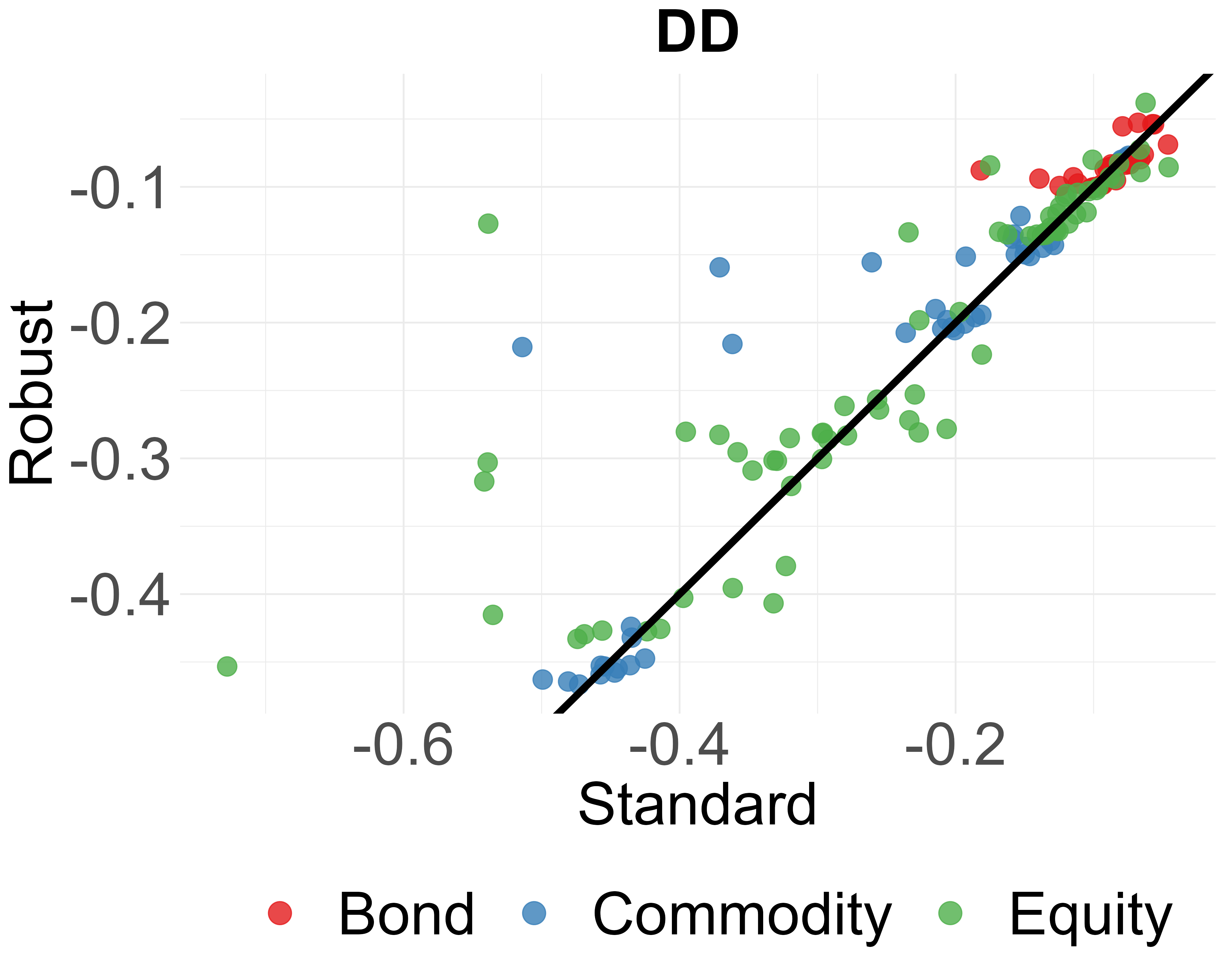
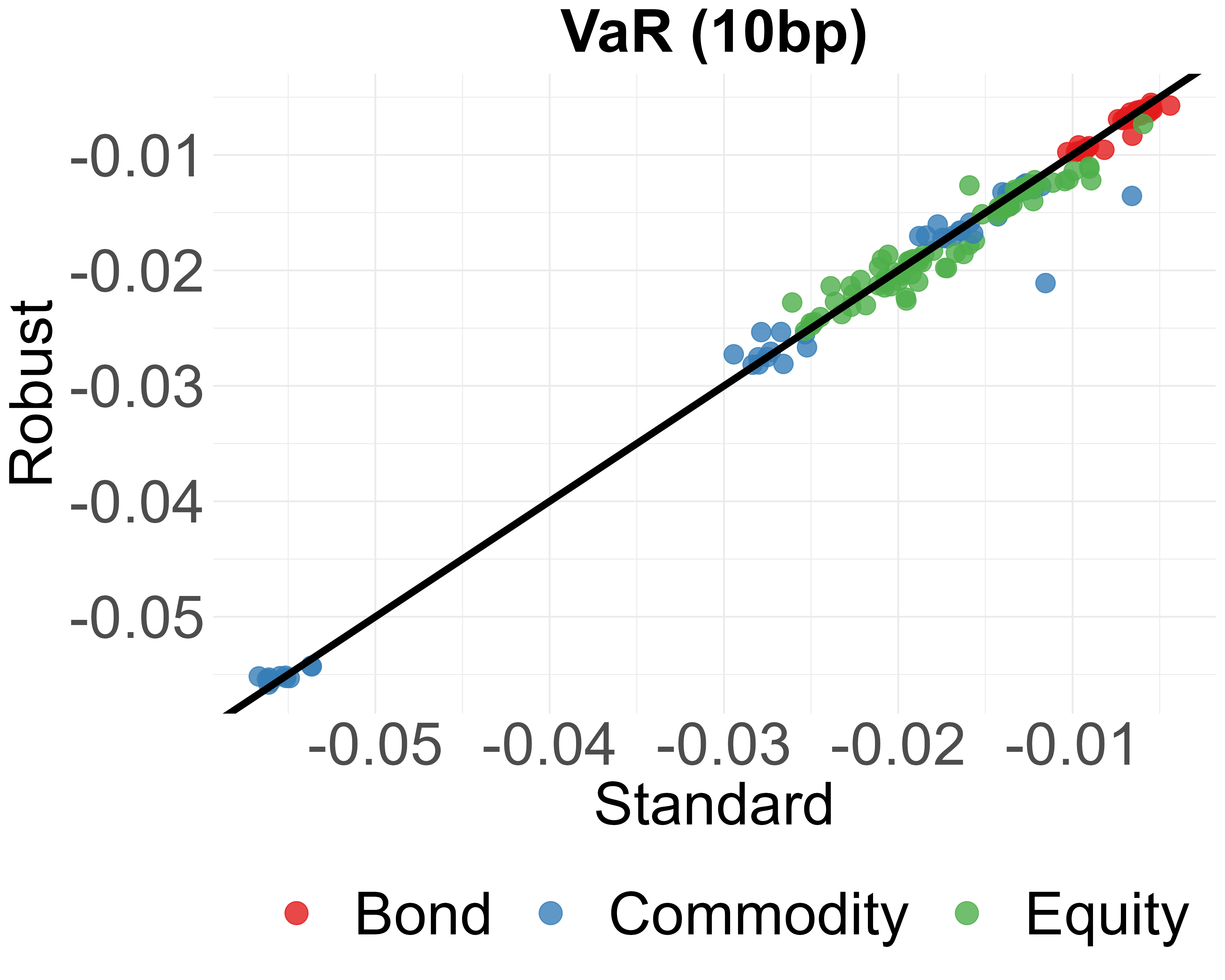
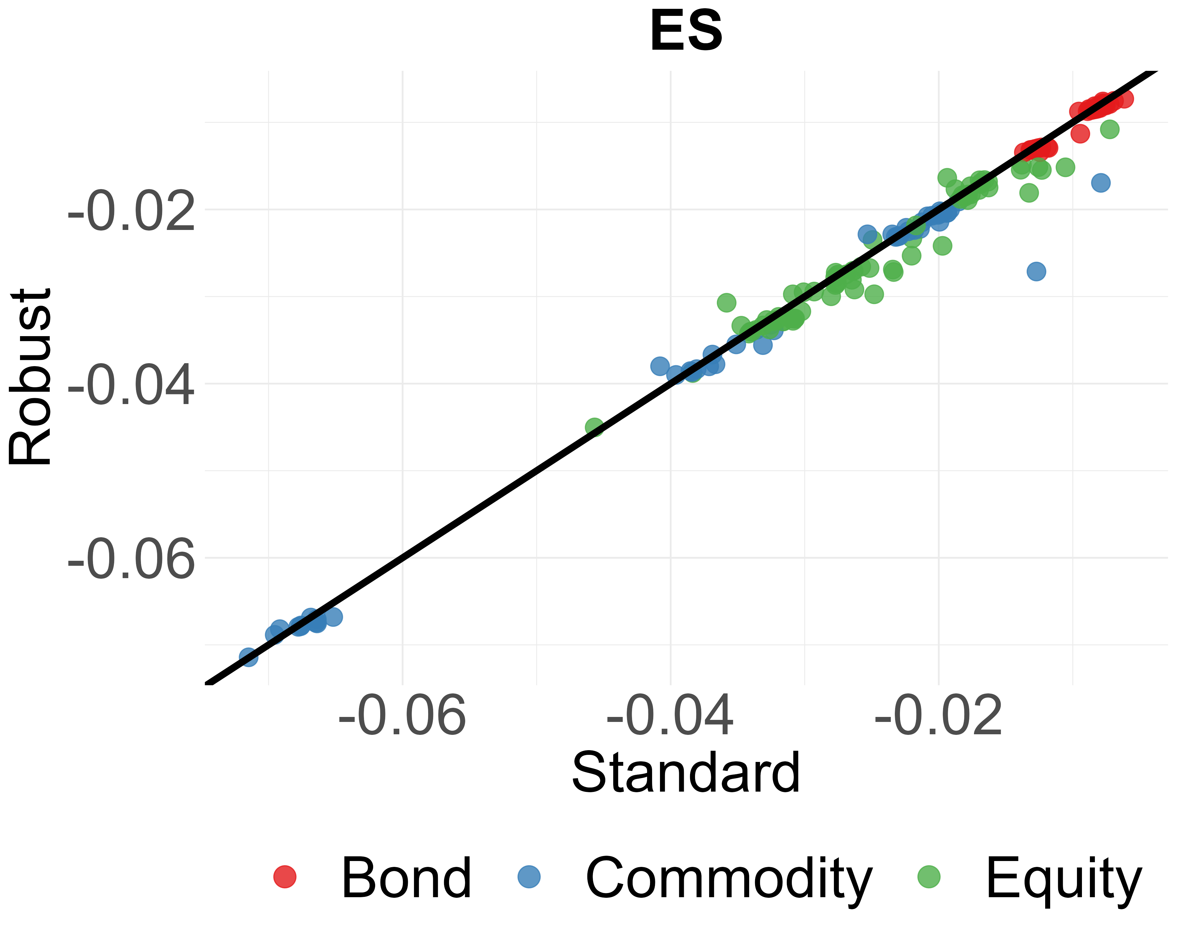
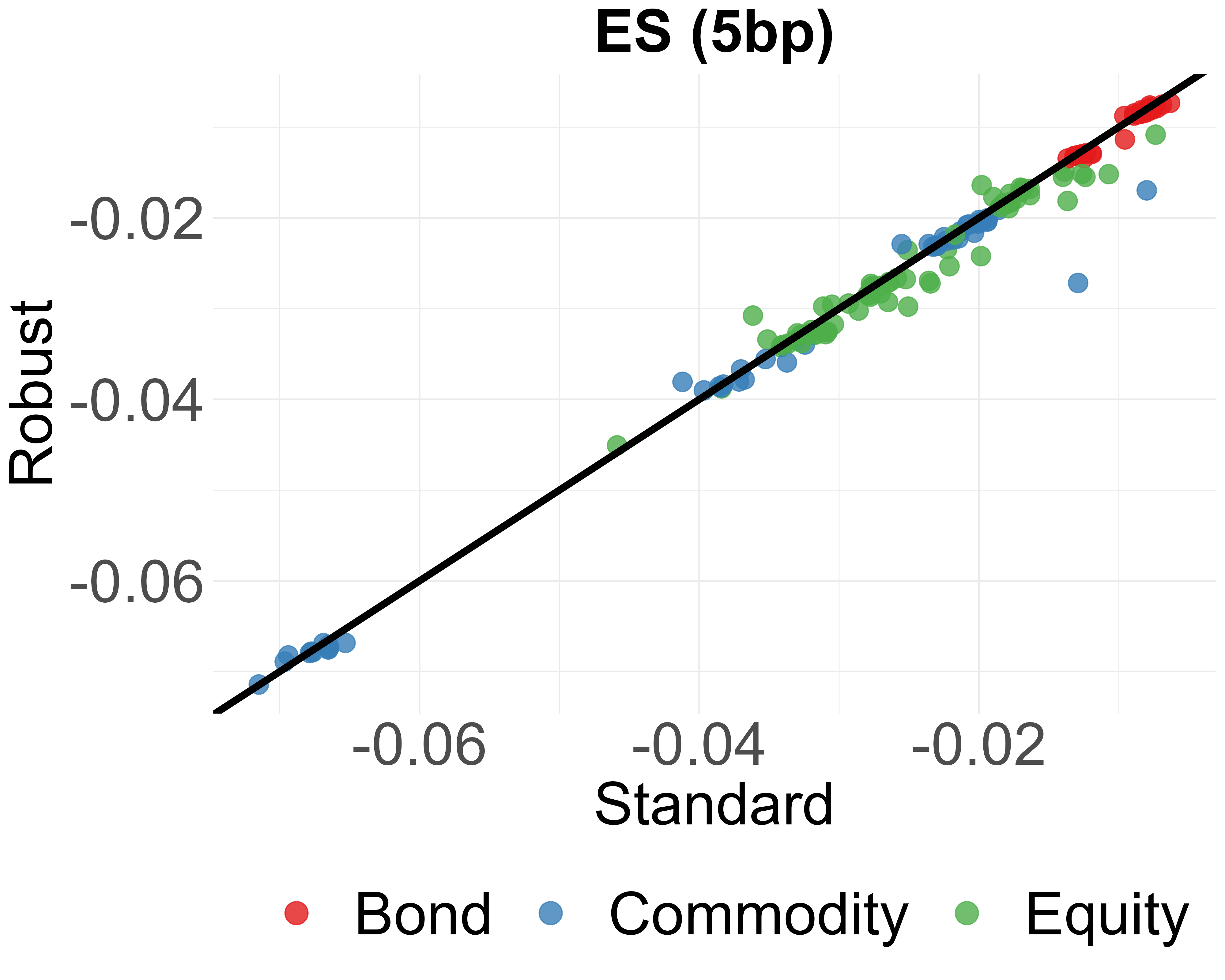
- Risk of big losses (drawdown, Value at Risk, Expected Shortfall)
- They also use bootstrap tests (a way of scrambling and resampling data) to check if the improvements are statistically meaningful and not luck.
What they found and why it matters
Here are the key results:
- More stable hedge ratios
- The robust hedge ratios move less and are smoother over time. This means you trade less often.
- Lower turnover and lower costs
- Because you’re trading less, you pay fewer transaction costs—an important win in real-life investing.
- Similar overall risk reduction, better protection when it matters most
- The robust method reduces overall variance about as well as standard methods.
- But it does better during bad market moments (downside protection), when investors most need the hedge.
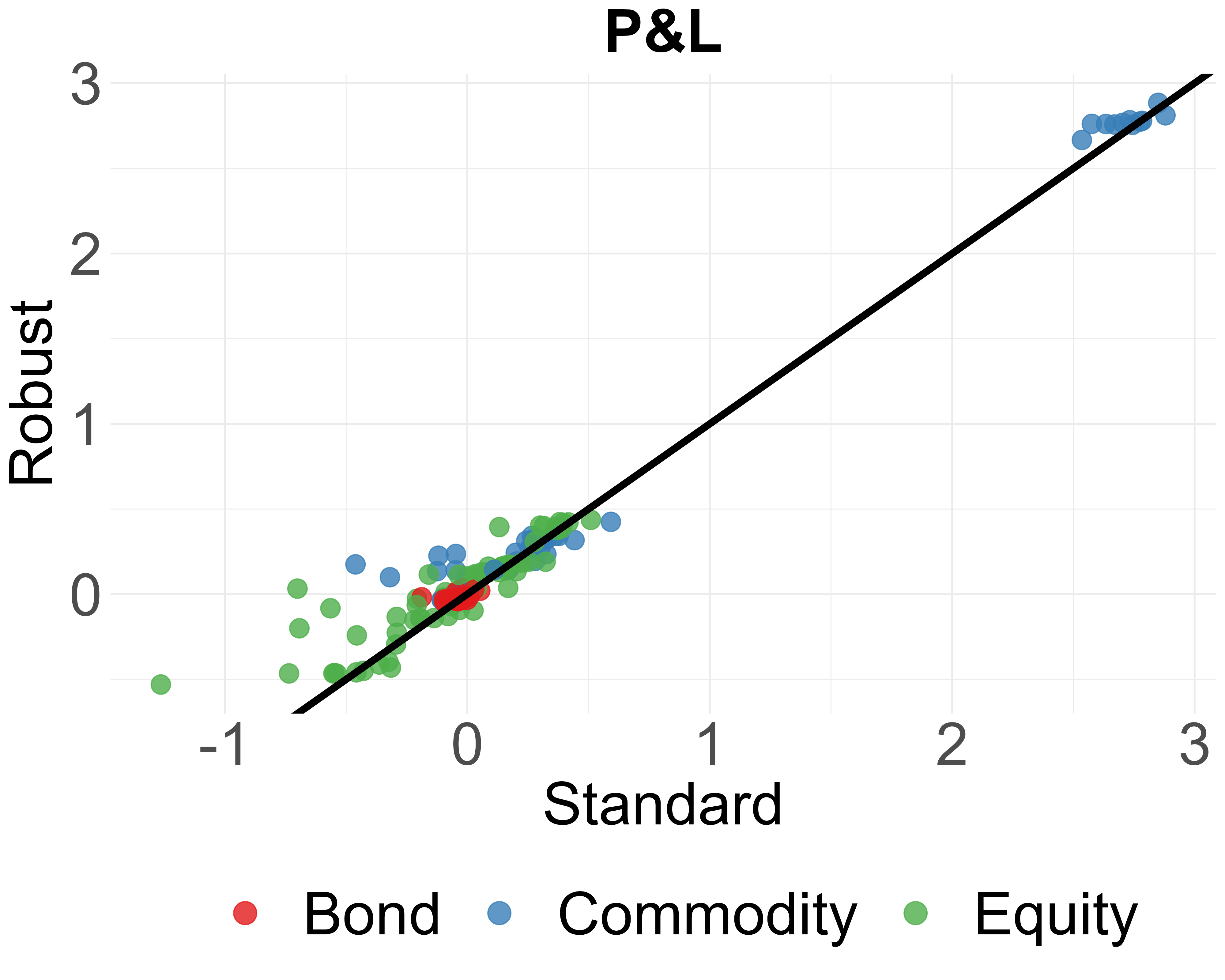
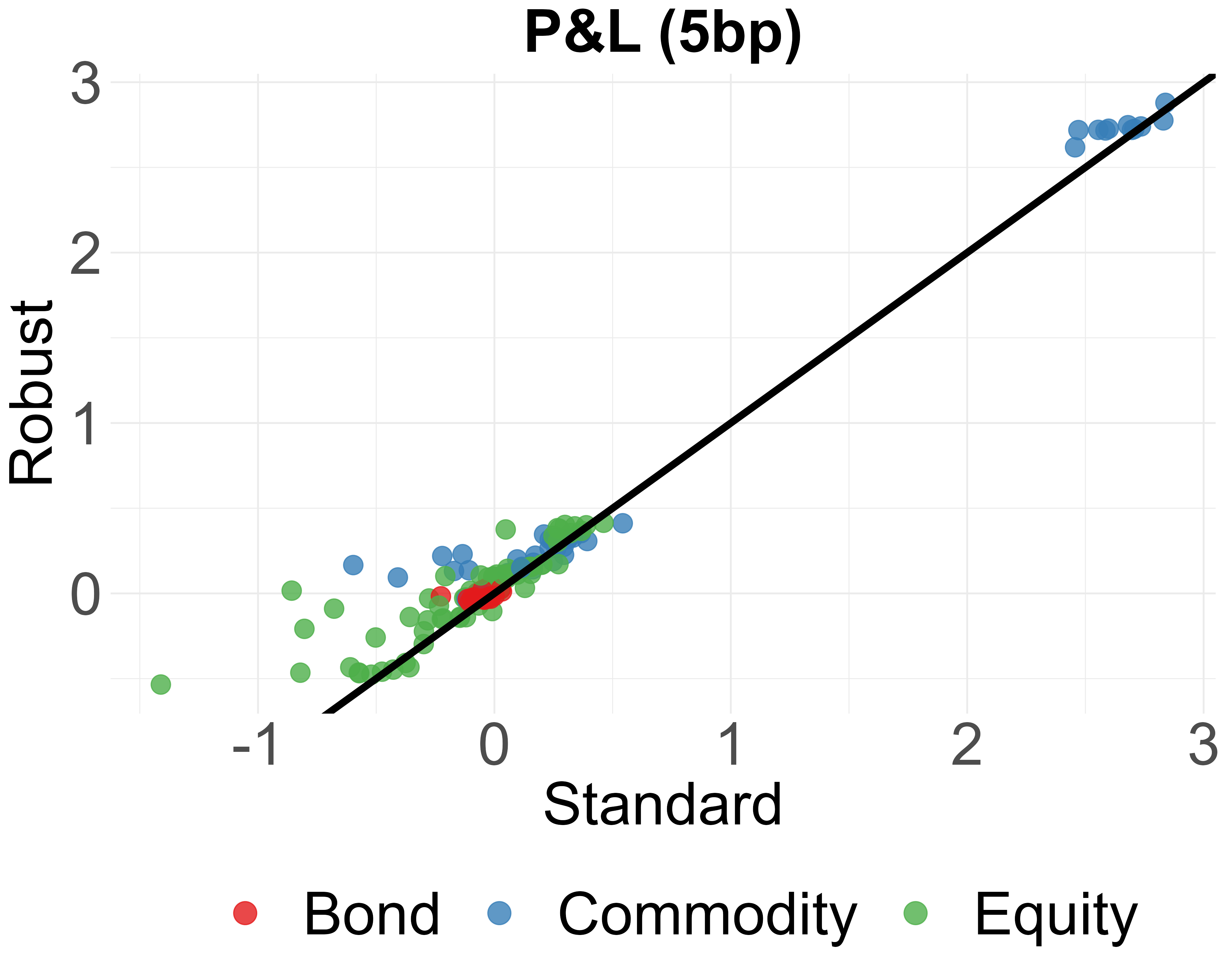
- Better risk-adjusted performance, especially after costs
- The robust method often leads to higher risk-adjusted returns (like better Sharpe and Omega ratios), particularly when you include trading costs.
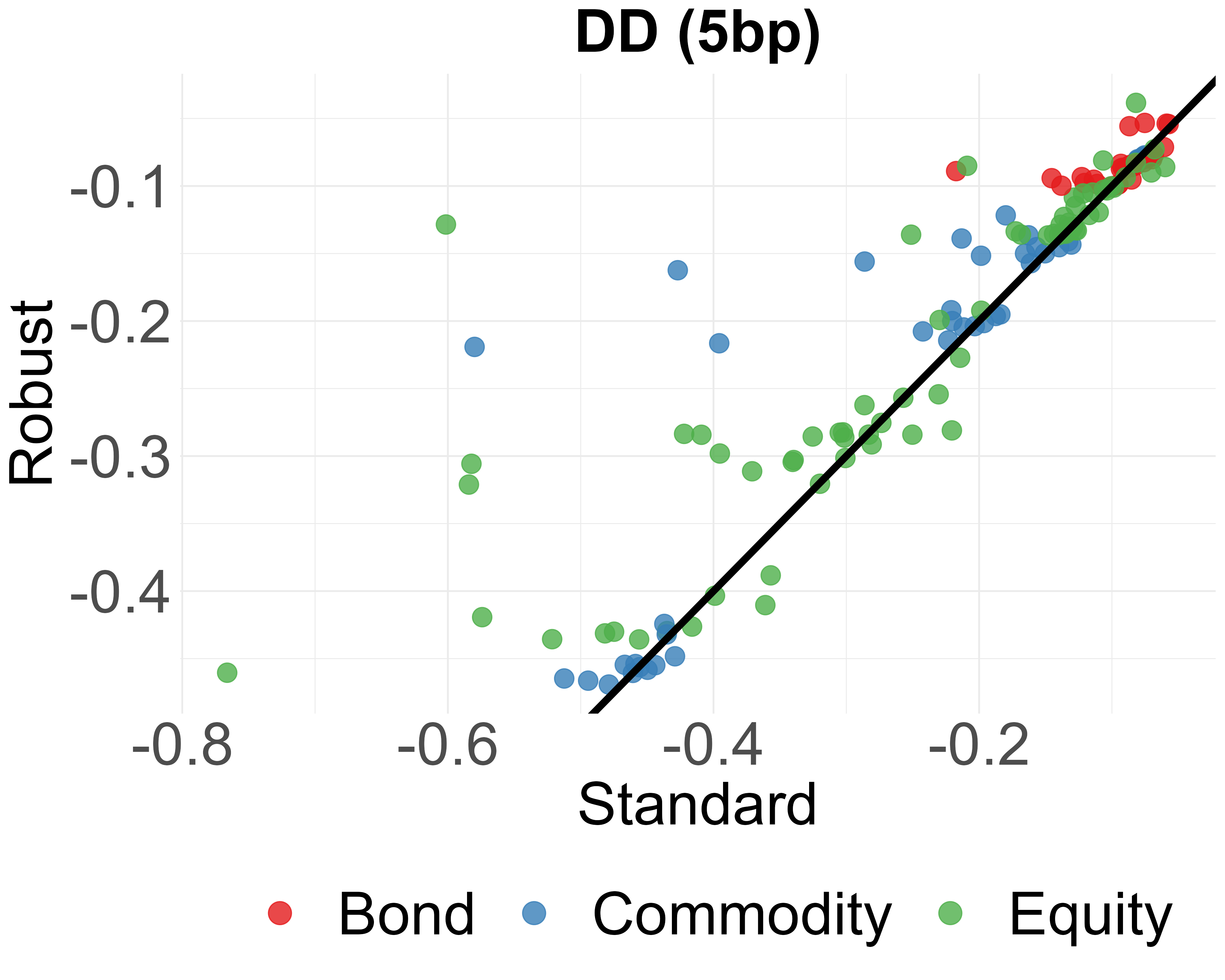
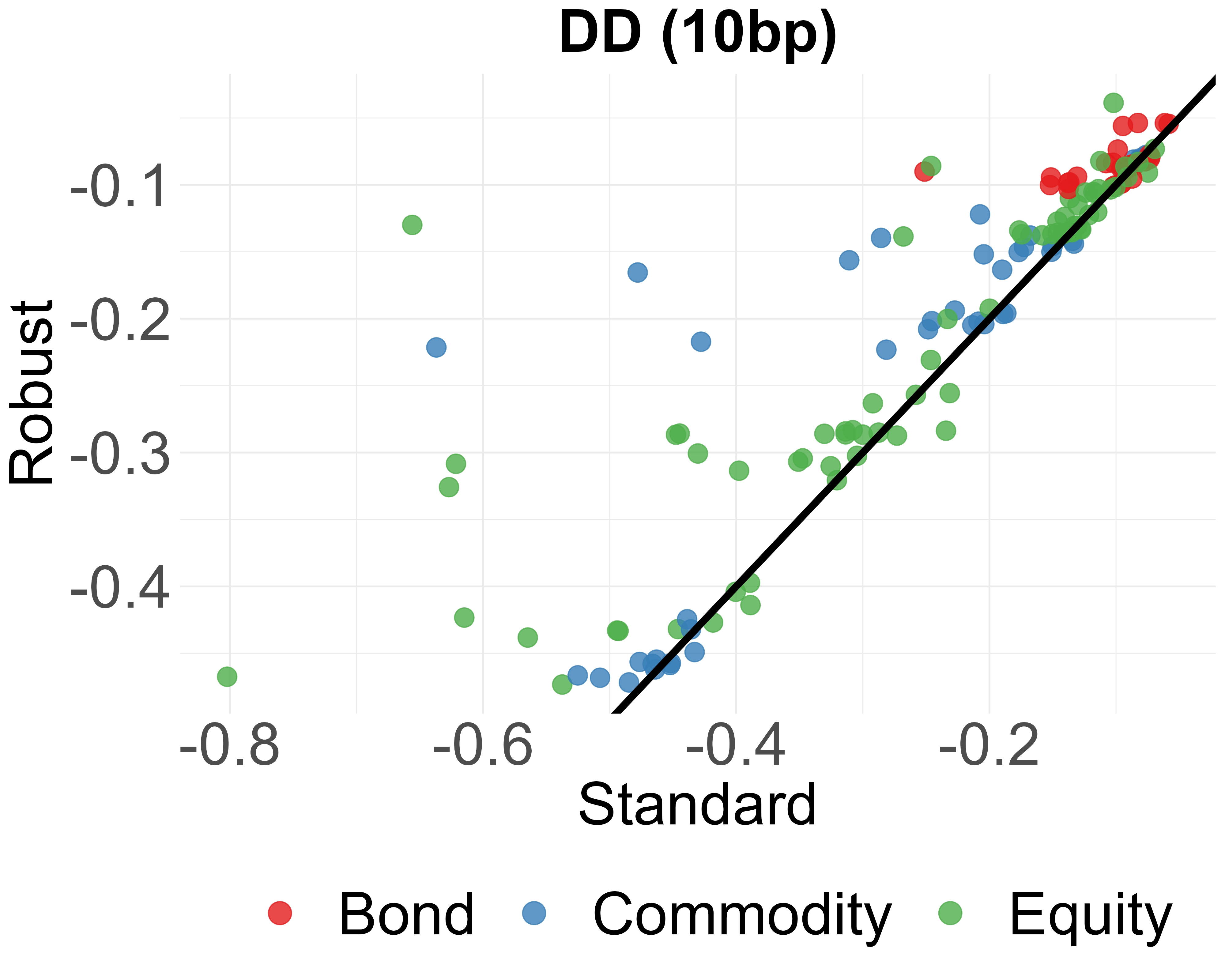
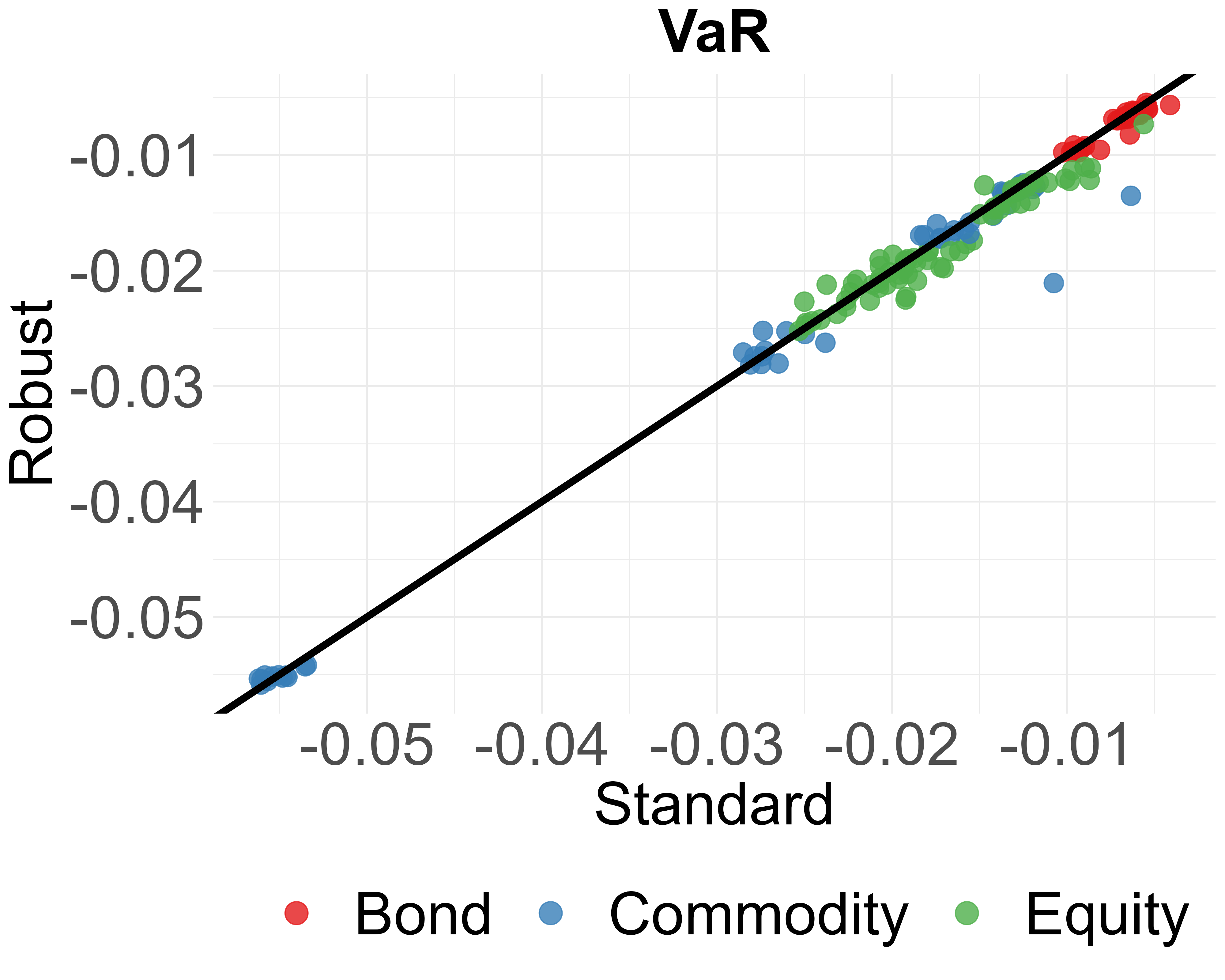
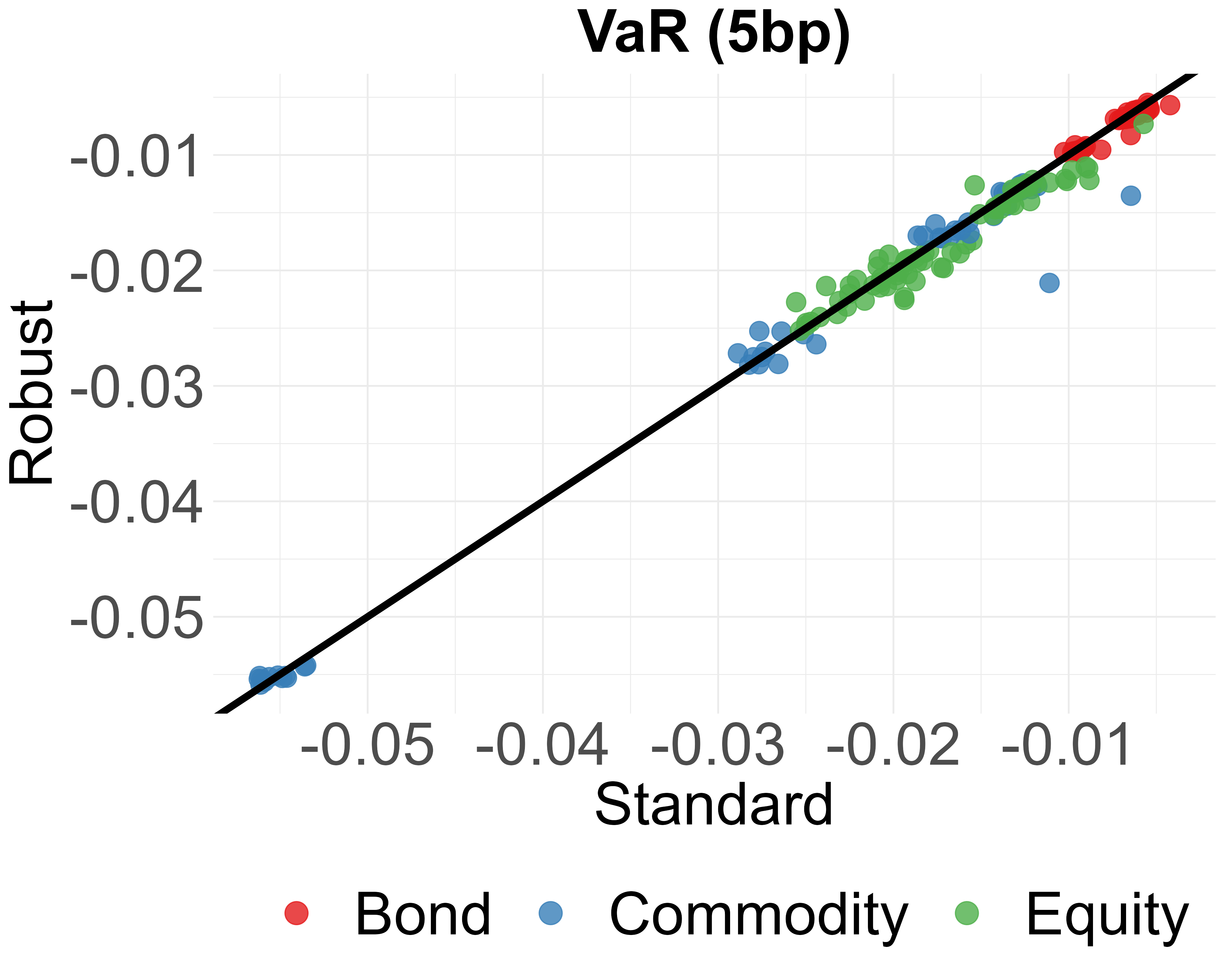
- It also tends to reduce large losses (lower drawdowns) and slightly improves tail-risk measures (VaR, Expected Shortfall).
- Results hold across many assets and tests
- The improvements are strongest for some asset pairs (like equities and gold), and mixed for others (like certain bond or clean energy pairs), but overall the robust approach shows clear benefits.
- Bootstrap checks support that these gains are statistically significant.
- Practical tips from their tests
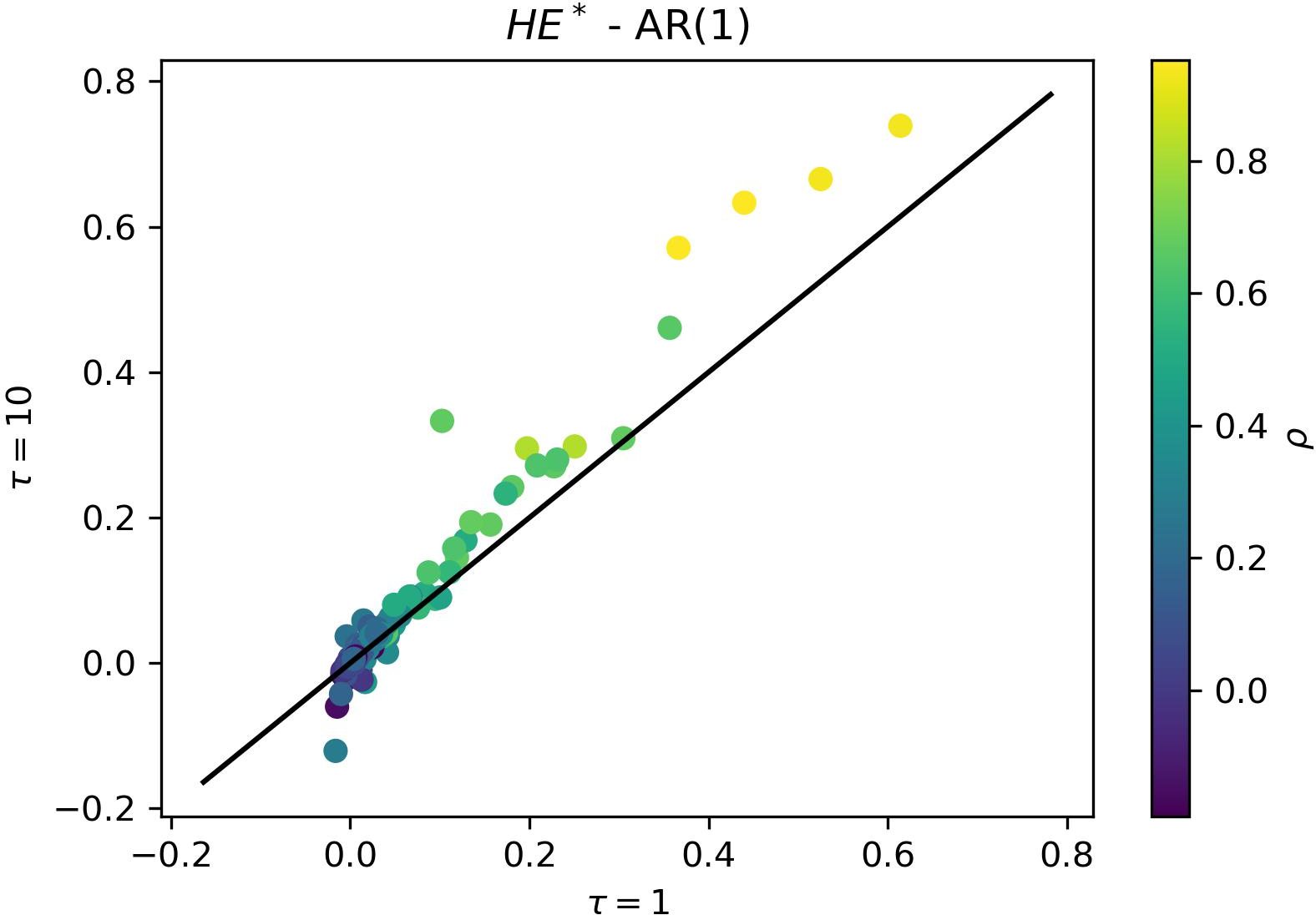
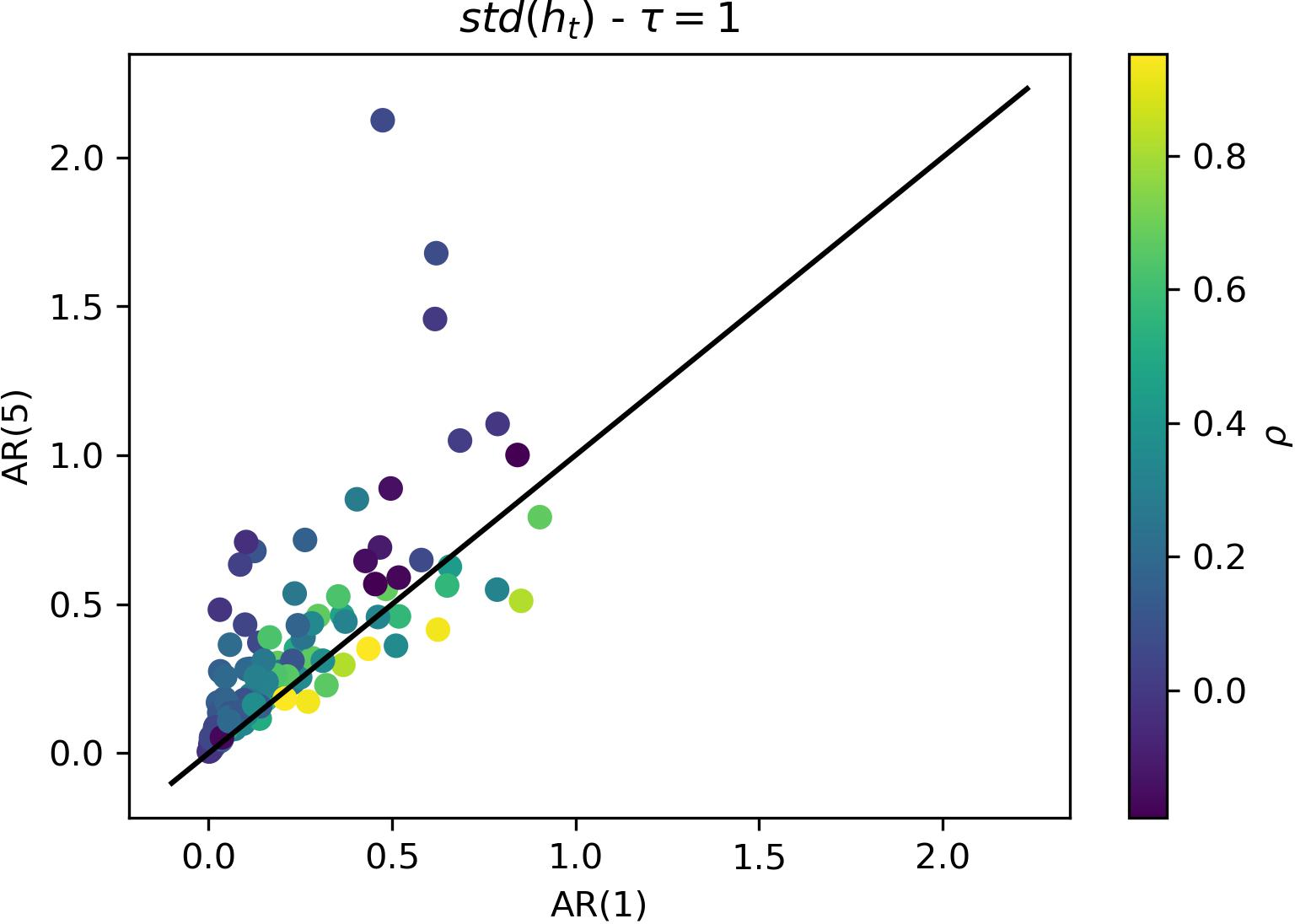
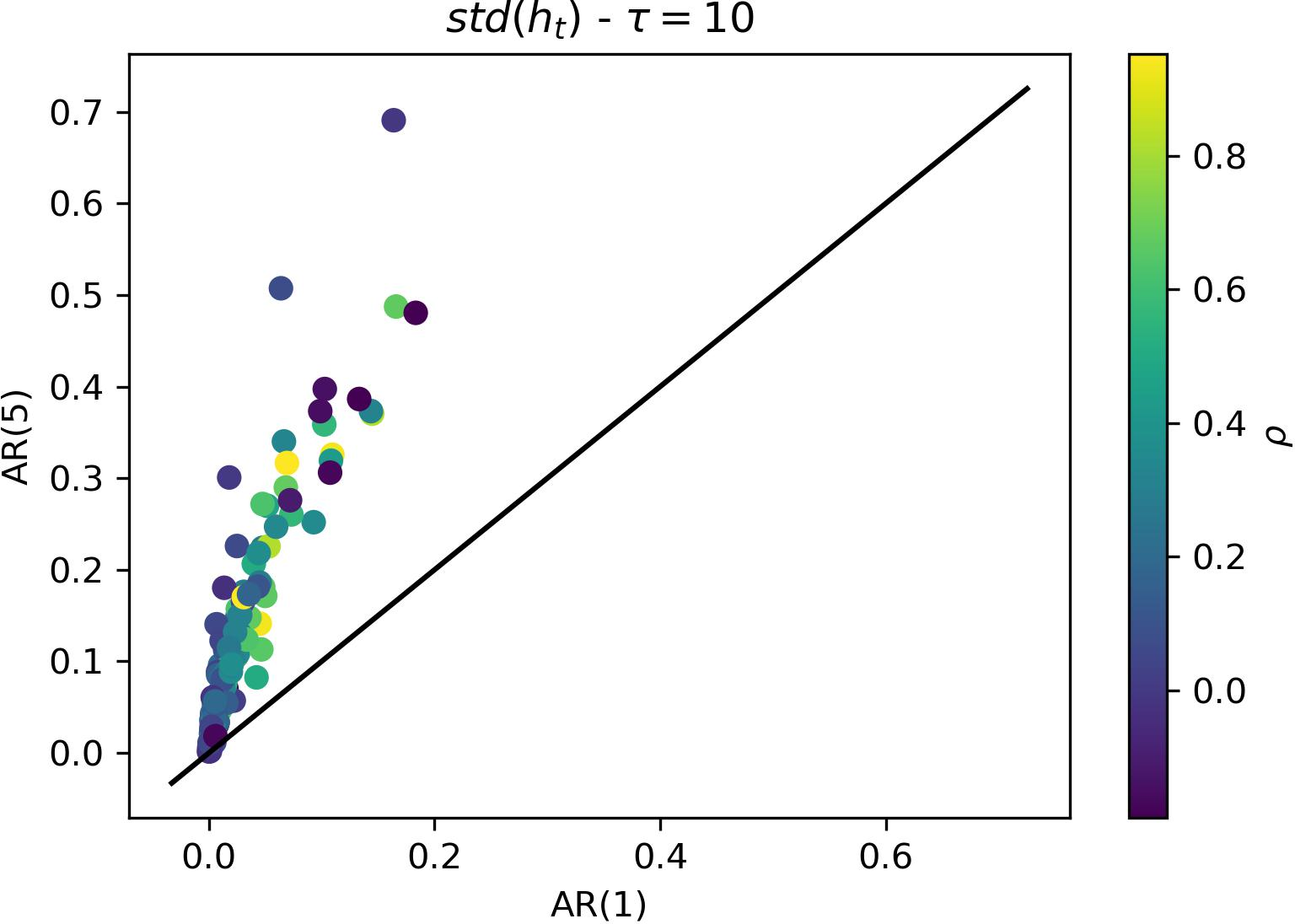
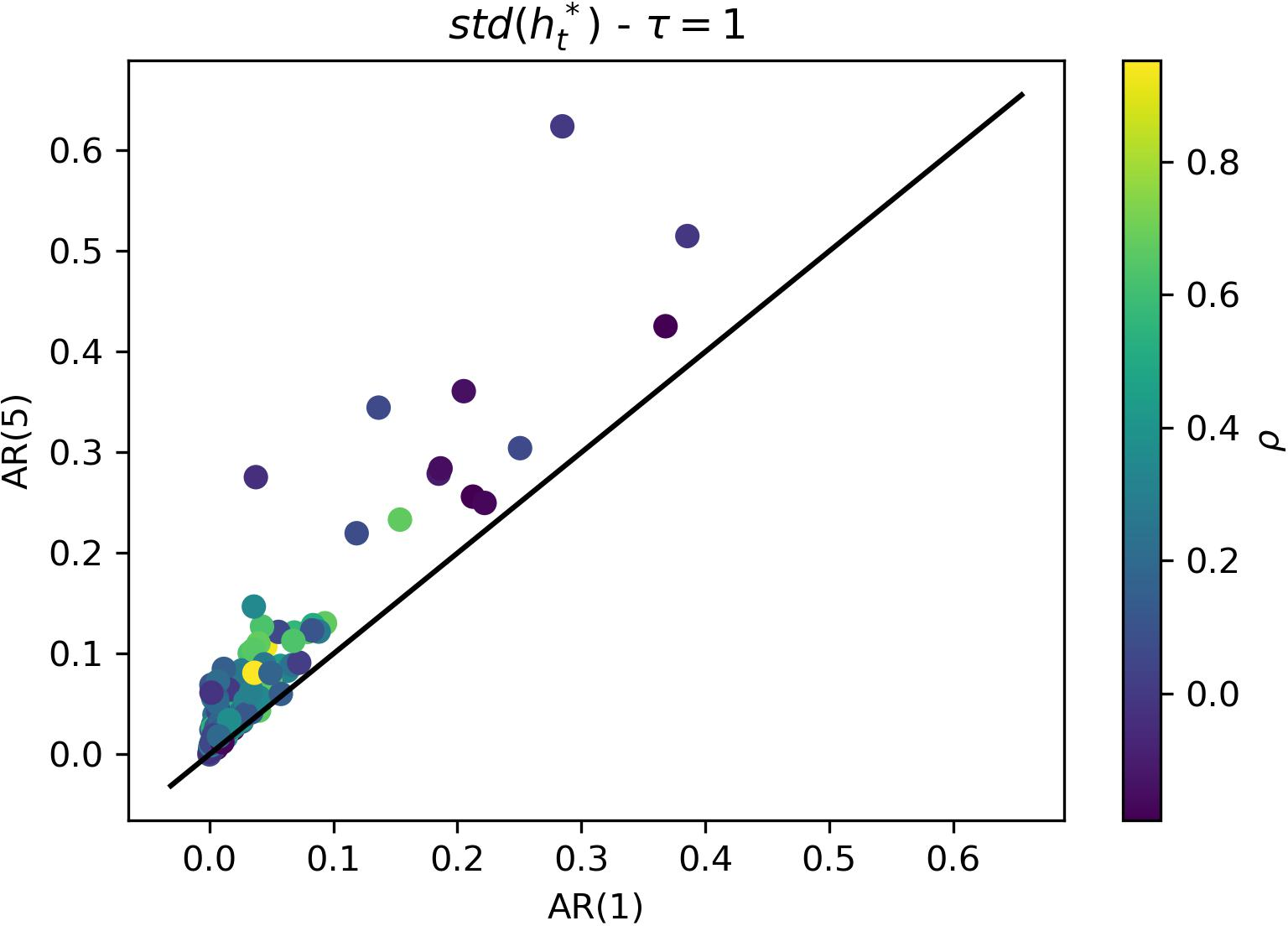
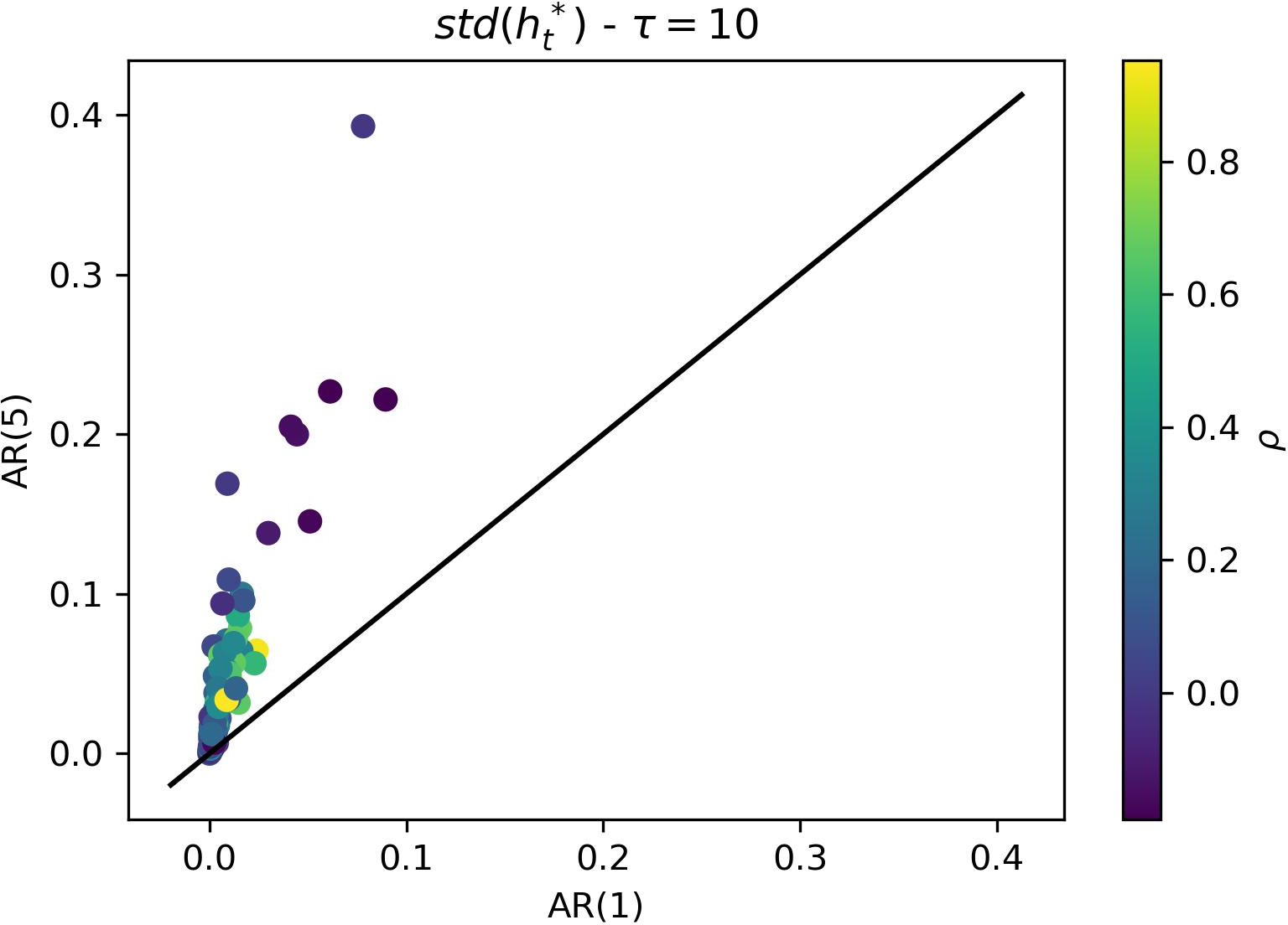
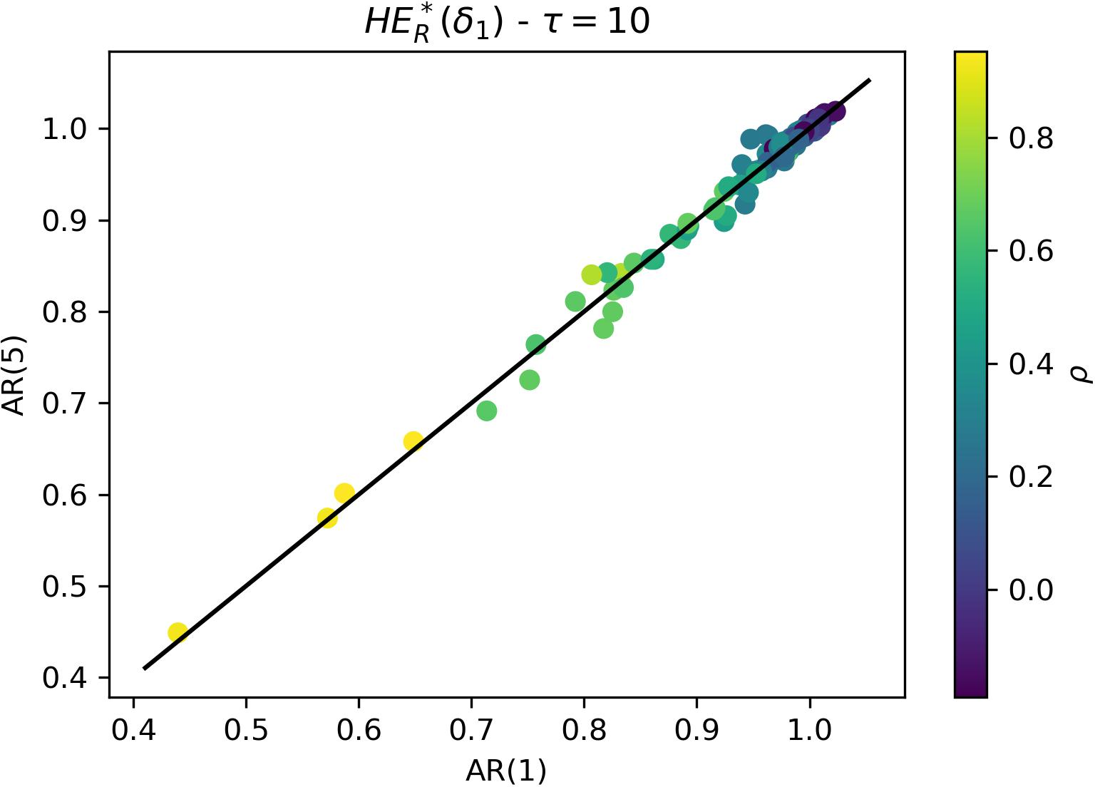
- Using longer forecasting horizons (e.g., planning hedge ratios every few days instead of daily) can reduce how much the hedge ratio bounces around, though it might slightly change how the hedge behaves in the worst cases.
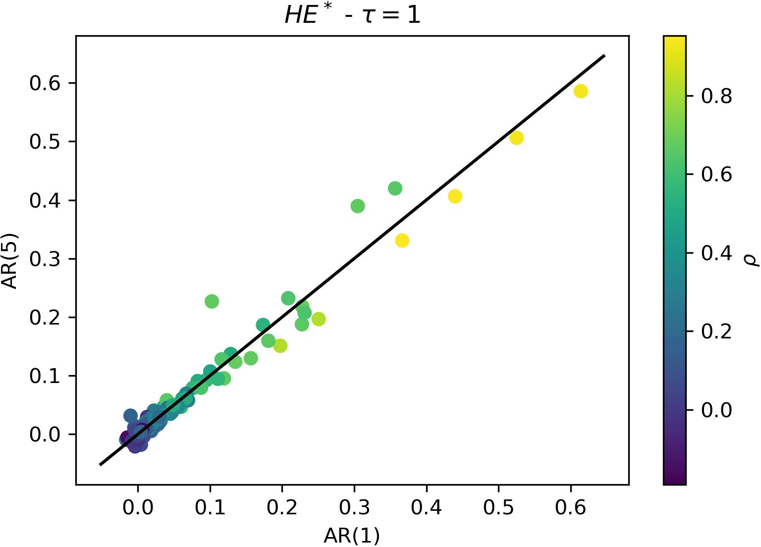
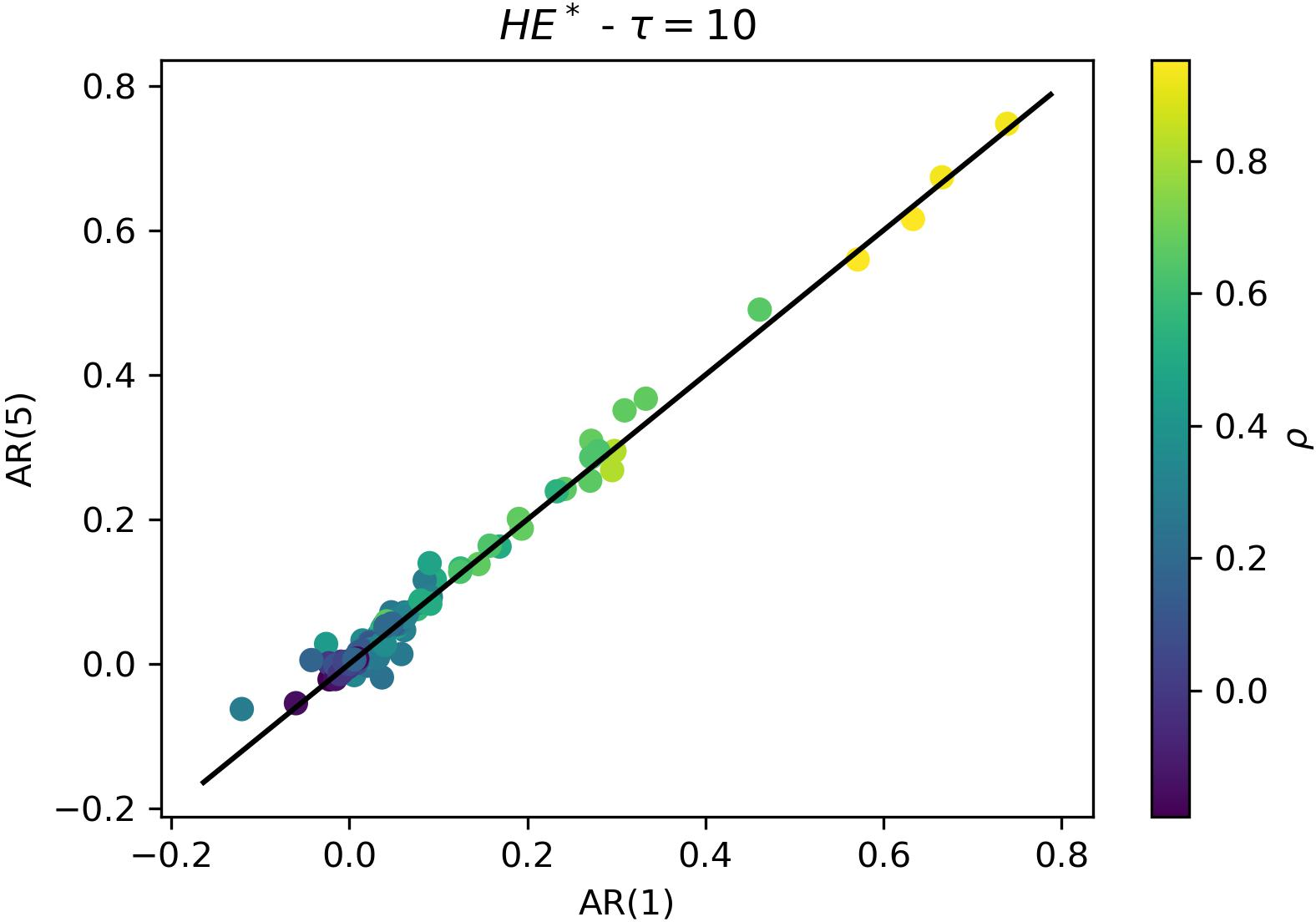
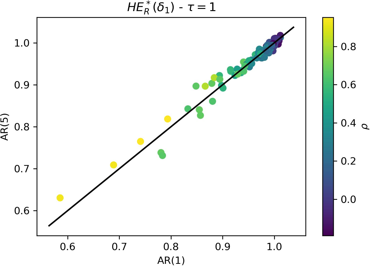
- Using more complex memory in forecasting (like AR(5) instead of AR(1)) can add complexity and sometimes more variability without big gains in effectiveness.
Why this is useful
For investors and risk managers:
- You get a hedge that’s calmer and cheaper to maintain.
- You keep most of the benefits of standard hedging while gaining better protection in bad times.
- You can implement this with simple, fast models and real market data.
- It works across different asset types and holds up under rigorous testing.
Final takeaway
The paper shows a practical, easy-to-use way to build hedges that plan for uncertainty. By combining high-frequency risk measures, simple forecasting, and a “safety margin” for forecast errors, the authors deliver hedge ratios that are steadier, cheaper to maintain, and often safer—especially when markets get rough. This approach can help both professionals and advanced individual investors manage risk more reliably without making their portfolios overly complicated.
Knowledge Gaps
Knowledge gaps, limitations, and open questions
Below is a consolidated list of what the paper leaves missing, uncertain, or unexplored, framed to be directly actionable for future research.
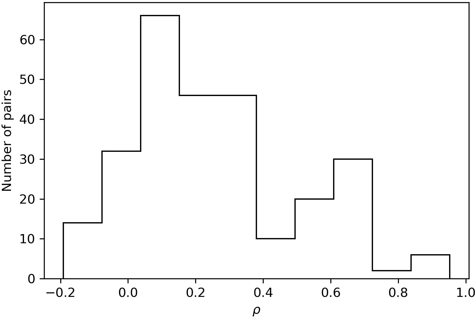
- Covariance/correlation uncertainty omitted: The robust set only covers variances; the covariance is treated as fixed (with ρ estimated in-sample). Quantify performance sensitivity to correlation misspecification and develop robust hedge ratios that also account for covariance (or correlation) uncertainty.
- Internal consistency of inputs: σSF is defined as ρσSσF yet treated as fixed while σS and σF vary within uncertainty sets. Clarify and test alternative formulations where σSF co-moves with variances (e.g., robust sets in (σS, σF, ρ) jointly).
- Calibration of uncertainty radius Θ: Θ is tied to AR forecast error dispersion but not mapped to a target confidence level. Establish a principled calibration (e.g., k-sigma, quantile-based) and study out-of-sample sensitivity of performance to Θ.
- Alternative uncertainty sets: Only box sets are considered. Compare ellipsoidal/budgeted sets and distributionally robust ambiguity sets (e.g., Wasserstein, φ-divergence) in terms of tractability, turnover, and tail protection.
- Forecasting model risk and structural breaks: AR(p)/HAR are used with the assumption of small estimation error. Evaluate robustness to parameter uncertainty, regime shifts, and model misspecification; benchmark against DCC-/GO-GARCH, realized-MIDAS, state-switching, and ML methods.
- Realized measure construction and microstructure noise: RV/RCV are built from 5-min returns without noise-robust methods. Test pre-averaging, subsampling, realized kernels, and multivariate noise-robust covariance estimators; quantify the impact of dropping the first/last half-hour and excluding overnight returns.
- Multi-horizon forecasting consistency: The paper sums one-step forecasts to form τ-step variances; analogous treatment for covariances and their uncertainty is not detailed. Derive joint multi-horizon forecast/uncertainty for both variances and covariances and assess overlapping-horizon effects.
- Unconstrained optimization vs practical constraints: The hedge problem is unconstrained. Extend to include leverage/short-sale/margin constraints and position bounds; study how constraints alter the robust solution and turnover.
- Transaction cost modeling: Costs are linear, constant bps per unit turnover. Incorporate spread- and volatility-dependent costs, nonlinear price impact, liquidity regimes, borrow fees for shorts, and slippage; assess how cost-aware robust objectives change hedging.
- Baseline comparisons: The empirical evaluation lacks head-to-head benchmarking versus widely used dynamic hedging methods (rolling OLS/Kalman beta hedges, DCC/BEKK hedges, shrinkage or ridge-regularized MV hedges, Bayesian hedging). Add these to contextualize gains.
- Objective choice vs tail risk: The optimization minimizes variance but tail metrics (VaR/ES) are only evaluated ex-post. Formulate and test robust objectives targeting CVaR/ES or downside variance; study trade-offs with turnover.
- Single-asset, single-hedge scope: The framework hedges one asset with one instrument. Generalize to multi-asset portfolios with multiple hedging instruments and cross-constraints; evaluate diversification and computational scalability.
- Endogenous rebalancing horizon: τ is varied but not optimized. Develop rules to choose τ dynamically (e.g., as a function of Θ, liquidity, or cost-benefit signals) and quantify performance-turnover trade-offs.
- Regime/state dependence: Performance heterogeneity across asset classes (e.g., bonds, clean energy) suggests state dependence. Introduce regime-switching/market-state-dependent Θ and test robustness through stressed periods beyond 2016–2024.
- ETF-specific basis/tracking risk: Hedging with ETFs introduces tracking error (e.g., roll, replication, cash drag). Measure basis risk and examine whether results generalize when hedging with futures or swaps.
- Bootstrap and inference design: Significance relies on 250-day blocks and MEB; sensitivity to block length, overlapping windows, and dependence across many pairwise tests is not explored. Add multiple-testing adjustments and robustness to resampling choices.
- Adaptive learning: Clarify whether model parameters and Θ are updated online. Investigate rolling/recursive estimation, time-varying Θ tied to volatility-of-volatility, and adaptive shrinkage of hedge ratios.
- Nonlinearity and jumps: Linear AR models and box sets may under-represent jumps/leverage effects in (co)volatility. Incorporate jump-robust realized measures and jump-diffusion/Hawkes dynamics, and design uncertainty sets capturing jump risk.
- Data quality and missingness: The M/Mt scaling addresses missing intraday bars, but the impact of outages/halts is not assessed. Stress test robustness under realistic missing-data mechanisms and apply microstructure-informed imputation.
- Theoretical guarantees: Provide finite-sample or probabilistic guarantees linking Θ to out-of-sample variance reduction and turnover bounds; derive regret or performance bounds under specified uncertainty.
- Closed-form generalization: The closed-form robust hedge depends only on ΘF. Investigate whether including ΘS and covariance uncertainty admits tractable solutions and specify sufficient conditions for uniqueness/global optimality with richer uncertainty sets.
- Nonlinear exposures: The method targets linear hedges for linear exposures. Extend to delta–gamma (or vega) robust hedging for options and convex payoffs with uncertain Greeks and volatility.
- Economic frictions: Net performance excludes taxes, funding costs, margin requirements, and capital charges. Quantify how these frictions alter the robust strategy’s net benefit.
- Intraday vs daily frequency: Only daily hedging is studied. Explore intraday rebalancing, different sampling frequencies (1–15 minutes), and frequency selection that balances noise and responsiveness.
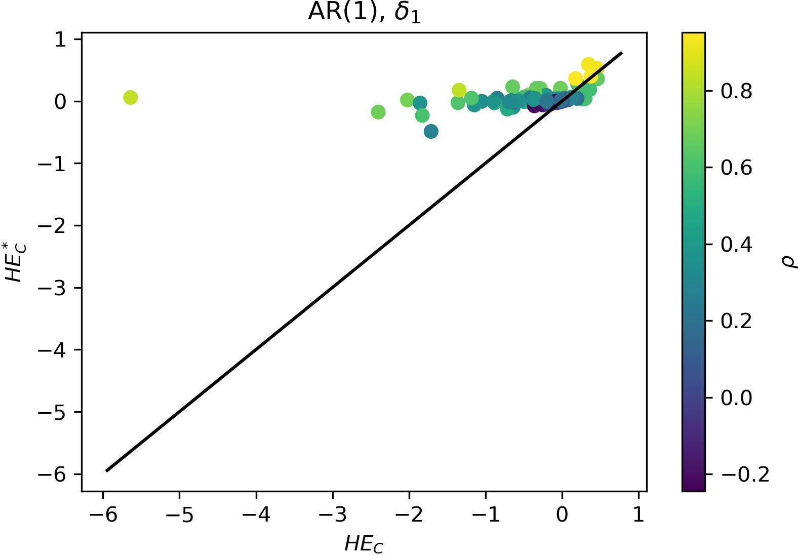
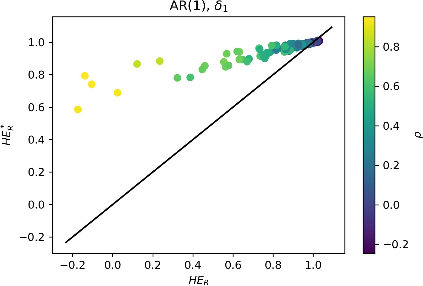
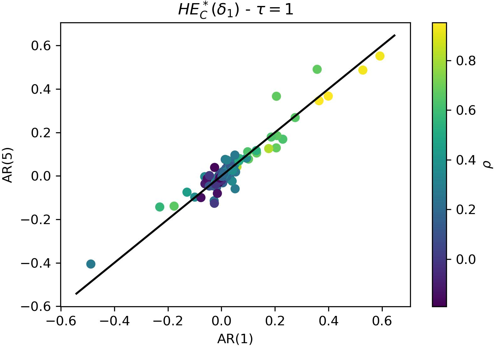
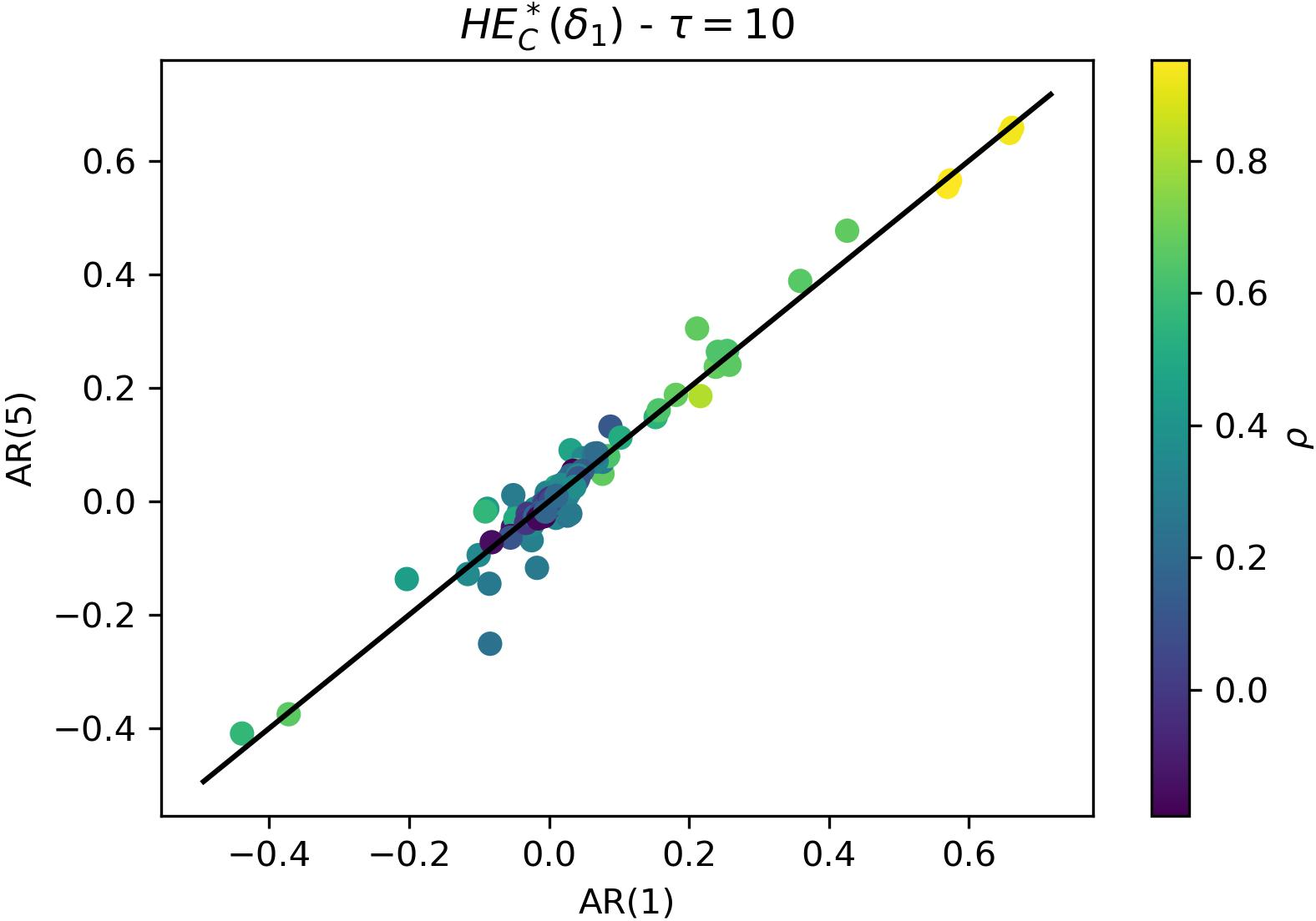
- Tail-conditioning design: Conditioned metrics HE_C and HE_R depend on δ (first quartile in plots). Systematically assess alternative thresholds, data-driven δ selection, and economic interpretation across assets/time.
- Lag vs responsiveness trade-off: Reduced turnover may delay responses to sudden regime shifts. Analyze drawdown and tail behavior around abrupt correlation spikes and design adaptive mechanisms to relax robustness when rapid adjustment is needed.
Practical Applications
Below is an overview of actionable, real-world applications that follow from the paper’s findings and methods. Each item specifies where it applies, how it could be implemented, and what assumptions or dependencies affect feasibility.
Immediate Applications
- Cost-aware dynamic hedging overlay for ETFs and single-asset exposures (Finance: asset management, hedge funds, wealth/robo-advisors)
- How to implement now: Replace standard minimum-variance hedge ratio with the paper’s robust hedge ratio h* using intraday realized variance/covariance, AR(p)-based multi-step forecasts, and box-uncertainty for variance. Rebalance on daily/weekly horizons τ selected to trade off turnover and protection.
- Tools/workflows: “Robust Hedging Engine” microservice that (i) ingests high-frequency data, (ii) computes RV/RCV, (iii) fits AR(p) on log-RV with bias correction, (iv) forecasts τ-step RV/RCV, (v) computes forecast-error-driven Θ and h*, (vi) emits signals to OMS/EMS with a no-trade band to control turnover.
- Assumptions/dependencies: Access to quality intraday data; liquid hedging instruments (e.g., futures/ETFs); transaction cost model calibrated in bps; shorting/borrowing permitted; box-uncertainty calibrated from forecast error; covariance uncertainty treated as negligible (per paper).
- Cross-hedging for commodity producers/consumers (Energy, Airlines, Agriculture, Industrials)
- How to implement now: Use robust hedge ratios to hedge oil, gas, jet fuel, and agricultural exposures with related futures/ETFs, emphasizing lower turnover and stability through τ>1 forecasts.
- Tools/workflows: Treasury/risk desk adds a robust hedging module to existing SAP/TMS; daily batch that updates RV/RCV from 5-min data, computes h*, and triggers hedges within pre-set band.
- Assumptions/dependencies: Basis risk remains; covariance assumed known; need liquid cross-hedges; intraday data may be proxied by exchange-traded futures even if physical exposure is off-exchange.
- FX and rate hedging with reduced rebalancing (Finance: corporates, pensions, insurers, LDI desks)
- How to implement now: Apply robust h* to FX forwards and interest-rate futures to hedge revenues, costs, or liabilities; target re-hedging on weekly cycles to cut turnover costs while preserving worst-case protection.
- Tools/workflows: Add robust hedge computation to LDI/ALM pipeline; dashboards show HE, HE_C, turnover, VaR/ES differentials from standard hedging.
- Assumptions/dependencies: Sufficient frequency data for rate/FX proxies (futures, liquid ETFs); funding/margin availability; policy tolerances for variance vs. downside risk.
- Pairs trading and market-neutral strategies with stable betas (Finance: hedge funds, prop trading, quant desks)
- How to implement now: Replace OLS/DCC-derived dynamic hedge ratios in pairs trades with robust h* to mitigate estimation risk and reduce over-trading.
- Tools/workflows: Integrate h* into spread/alpha construction; add no-trade bands and τ-step horizons to smooth signals; evaluate with bootstrap significance as in paper.
- Assumptions/dependencies: Strategy alpha not degraded by slightly slower adjustments; availability of intraday data for RV/RCV; stability benefits outweigh small loss in variance-fit.
- Broker/robo-advisor “defensive overlay” for retail portfolios (Finance: wealth tech)
- How to implement now: Offer an optional hedging overlay that uses robust h* with low turnover to protect against left-tail moves; communicate improved drawdown and ES profiles, net of costs.
- Tools/workflows: API that computes h* for each eligible client sleeve (e.g., equity sleeve hedged with index futures/ETFs) using standardized τ and Θ calibration; compliance-aligned client disclosures.
- Assumptions/dependencies: Suitability and KYC constraints; transparent cost modeling; adequate liquidity in retail-accessible hedges (e.g., liquid ETFs).
- Risk reporting and governance upgrade (Finance: risk/compliance functions)
- How to implement now: Add HE_C and HE_R as downside-focused hedge effectiveness KPIs; track turnover and transaction-cost-adjusted Sharpe/Omega differentials between standard and robust hedges.
- Tools/workflows: Risk dashboards that plot h*, HE, HE_C, HE_R, turnover, VaR/ES; bootstrap-based significance panels as in the paper to validate performance differences.
- Assumptions/dependencies: Data engineering for intraday inputs; governance on Θ calibration and τ/AR order selection; model documentation for auditability.
- Curriculum and replication packages (Academia/education)
- How to implement now: Use the paper’s framework as a teaching module in risk management and quantitative finance courses; provide code labs to compute RV/RCV, fit AR(p), and implement robust h* with transaction costs.
- Tools/workflows: Python/R notebooks; data from liquid ETFs/futures; assignments comparing standard vs. robust hedging with bootstrap inference.
- Assumptions/dependencies: Access to sample intraday datasets; pedagogical simplifications for students (e.g., pre-processed returns).
- Vendor/API offering for realized risk and robust hedging (Data/software vendors, fintech)
- How to implement now: Commercialize an API that streams RV/RCV, AR forecasts, Θ estimates, and robust h* across key assets and horizons τ.
- Tools/workflows: SLA-backed data ingestion, microstructure filters, model training pipelines, streaming endpoints, and alerting for threshold breaches.
- Assumptions/dependencies: Data licenses; latency and uptime SLAs; client integration with OMS/EMS.
Long-Term Applications
- Multi-asset robust hedging with covariance uncertainty and constraints (Finance: asset managers, banks)
- Future direction: Extend to vector hedging with multiple instruments, robustifying both variances and covariances (ellipsoidal/ambiguity sets, Bayesian posteriors), and adding liquidity, leverage, and regulatory constraints.
- Potential products/workflows: Multi-hedge optimizer that co-selects instruments, horizons, and rebalancing cadence; liquidity- and impact-aware robust hedging.
- Key dependencies: Computational scaling; reliable estimation of covariance uncertainty; integration with complex constraint sets and multi-market liquidity.
- High-frequency and microstructure-aware robust hedging (Finance: market makers, HFT, structured desks)
- Future direction: Bring robust hedging to intraday horizons using microstructure-noise-robust realized measures and adaptive τ; integrate execution cost models and market impact.
- Potential products/workflows: Co-optimized hedging and execution algorithm that balances h* tracking and impact; dynamic no-trade bands from real-time cost estimates.
- Key dependencies: Sub-minute data quality; robust microstructure filters; real-time risk-engine integration; more realistic cost/impact models.
- Robust hedging for options/greeks and nonlinear exposures (Finance: derivatives dealers, structured products)
- Future direction: Generalize the framework to hedging delta/vega/gamma exposures where both volatility and correlation forecasts are uncertain; combine with model-risk bounds.
- Potential products/workflows: “Greeks-robust” overlays for option books that reduce re-hedging churn while controlling tail risk; scenario-robust stress kits for implied vol surfaces.
- Key dependencies: Joint modeling of realized and implied volatility; covariance and correlation uncertainty; nonlinearity-aware robust optimization.
- Enterprise treasury platforms with robust hedging governance (Corporates: multi-national treasuries)
- Future direction: Enterprise-grade TMS modules embedding robust h*, policy-based rebalancing, and automated compliance checks across commodities, FX, and rates.
- Potential products/workflows: Policy engines that set τ and Θ based on exposure criticality; exception reporting; ESG-aligned hedge selection (e.g., green energy hedges).
- Key dependencies: Cross-entity data consolidation; internal controls and audit trails; cross-border regulatory compliance.
- Regulatory and supervisory toolkits (Policy/regulators)
- Future direction: Encourage or benchmark stress-resilient hedging by considering forecast uncertainty and turnover costs in hedge-effectiveness assessments and stress tests.
- Potential products/workflows: Supervisory templates that include HE_C/HE_R; scenario libraries that vary Θ and correlations; peer benchmarking of hedging stability.
- Key dependencies: Industry data collection; harmonized methodologies; alignment with accounting hedge-effectiveness rules.
- Retail “auto-hedge” offerings and retirement overlays (Wealth/retirement platforms)
- Future direction: Consumer-facing hedging overlays with explainable, low-churn robust h* for major risk sleeves (equity, duration, commodities); lifecycle-aware τ/Θ.
- Potential products/workflows: Opt-in features with guardrails; transparent cost disclosures; goal-based settings (e.g., drawdown caps).
- Key dependencies: Investor education; suitability/UX; fee models; ETF/futures access constraints.
- Cross-asset ESG/transition-risk hedging (Energy/utilities/real assets)
- Future direction: Robust hedging for transition exposures (e.g., carbon, power price volatility) where data and model uncertainty are pronounced.
- Potential products/workflows: Robust cross-hedges using correlated liquid proxies (e.g., carbon futures, power indices) with calibrated Θ from sparse data.
- Key dependencies: Data scarcity and liquidity; policy shifts affecting correlations; evolving market microstructure.
- Cloud-native “Robust Hedging as a Service” (Software/fintech)
- Future direction: Full-stack, multi-tenant service delivering robust h*, performance analytics, and governance logs, integrated with execution partners.
- Potential products/workflows: End-to-end connectors to brokers; configurable τ/AR order and Θ; integrated bootstrap-based significance reporting.
- Key dependencies: Security and compliance; interoperability with third-party OMS/EMS; client-specific customizations and SLAs.
Notes on feasibility and transferability across all applications:
- Data: The methodology relies on high-frequency realized measures; where intraday data are unavailable, proxies or lower-frequency variants can be used at some loss of responsiveness.
- Modeling: AR(p)/HAR model selection and Θ calibration (from forecast error variance) are critical; mis-calibration can lead to over/under-hedging.
- Assumptions: The paper’s main results assume negligible covariance uncertainty and focus on variance robustness; this can be conservative in regimes with correlation spikes.
- Costs and frictions: Transaction costs modeled as bps per turnover; further work is needed for comprehensive impact models (slippage, spreads, borrow costs).
- Scope: The framework targets minimum-variance objectives; if return forecasts or utility preferences matter, a mean–variance–cost robust extension may be needed.
Glossary
- AR(p) model: An autoregressive time-series model of order p used to forecast future values based on past observations. Example: "we consider an autoregressive model of order , namely an AR(p) model"
- Augmented Dickey–Fuller test: A statistical test used to assess whether a time series is stationary. Example: "we assess the stationarity of the resulting time series by means of Augmented DickeyâFuller tests."
- basis points (bp): One hundredth of a percentage point (0.01%), commonly used to quote costs or rates. Example: "bp denotes the transaction cost per unit of hedge ratio turnover in basis points."
- box uncertainty set: A rectangular (interval-based) set specifying independent bounds for uncertain parameters in robust optimization. Example: "As such, the box uncertainty set is defined as"
- box-uncertainty robust optimization scheme: A robust optimization approach that guards against worst-case outcomes within box-bounded parameter uncertainty. Example: "and a box-uncertainty robust optimization scheme."
- bootstrap: A resampling method used to assess statistical significance or variability of estimates. Example: "Bootstrap evidence supports the statistical significance of these gains."
- covariance matrix: A matrix capturing variances and covariances among multiple variables (here, asset returns). Example: "let be the covariance matrix between the returns of the two instruments over the portfolio time horizon "
- DCC-GARCH: Dynamic Conditional Correlation Generalized Autoregressive Conditional Heteroskedasticity; a multivariate volatility model with time-varying correlations. Example: "multivariate DCC-GARCH frameworks"
- downside protection: Strategies or features aimed at limiting losses during adverse market moves. Example: "the robust approach improves downside protection and risk-adjusted performance"
- error maximization: The amplification of portfolio weight instability due to input estimation errors. Example: "a phenomenon commonly referred to as estimation risk or error maximization"
- estimation risk: The risk arising from uncertainty or error in estimated model inputs. Example: "a phenomenon commonly referred to as estimation risk or error maximization"
- Expected Shortfall (ES): A tail-risk measure equal to the expected loss conditional on losses exceeding VaR at a given confidence level. Example: "the Expected Shortfall (ES) quantifies the average loss conditional on exceeding this threshold"
- HAR model: The Heterogeneous Autoregressive volatility model aggregating daily, weekly, and monthly components. Example: "the so-called HAR model can reproduce the stylized facts"
- hedge effectiveness (HE): A metric quantifying reduction in variance (or related measures) achieved by a hedging strategy. Example: "Hedge effectiveness () is a standard measure of hedging performance in this context"
- hedge ratio: The size of the hedging position relative to the exposure, chosen to minimize portfolio variance. Example: "Hedge ratios are fundamental tools in financial risk management"
- impulse response function: The dynamic response of a model variable to a shock over time. Example: "and the impulse response function."
- integrated variance: The sum of instantaneous variances over a horizon; a measure of cumulative volatility. Example: "it follows that the estimated volatility over a horizon is the square root of the integrated variance over steps"
- market impact: The price effect caused by trading activity, especially large or frequent trades. Example: "transaction costs, market impact, and operational complexity"
- market microstructure effects: Phenomena arising from the trading process and market design that affect prices and execution. Example: "and the interaction between robust hedging and market microstructure effects"
- maximum drawdown (DD): The largest peak-to-trough decline of a portfolio over a period. Example: "the maximum drawdown (DD) captures the largest observed decline from a portfolioâs peak to its subsequent trough"
- Maximum Entropy Bootstrap (MEB): A bootstrap method that preserves temporal dependence by resampling in a way consistent with maximum entropy principles. Example: "using the Maximum Entropy Bootstrap (MEB) of \citet{vinod2009maximum}"
- min-max problem: An optimization that minimizes an objective under the worst-case (maximum) realization of uncertainty. Example: "the following {\it unconstrained} min-max problem"
- minimum-variance (MV) hedging: A hedging approach that sets positions to minimize the variance of the hedged portfolio. Example: "dynamic minimum-variance hedging"
- Omega ratio: A performance metric comparing probability-weighted gains to losses relative to a threshold. Example: "the Omega ratio () compares probability-weighted gains and losses relative to a given benchmark"
- realized covariance (RCV): An ex-post high-frequency-based estimator of covariance from intraday returns. Example: "realized variance (RV) and realized covariance (RCV) estimators"
- realized variance (RV): An ex-post high-frequency-based estimator of variance from intraday returns. Example: "realized variance (RV) and realized covariance (RCV) estimators"
- robust optimization: Optimization that accounts for parameter uncertainty by safeguarding against worst-case scenarios. Example: "we embed forecasts into a robust optimization framework with box uncertainty sets for variances and covariances"
- Sharpe ratio: A risk-adjusted performance measure defined as excess return per unit of volatility. Example: "the Sharpe ratio (SR) is a measure of the risk-adjusted return of an investment"
- transaction costs: Costs incurred from trading, such as fees and bid-ask spreads, often modeled as proportional to turnover. Example: "This instability translates into substantial transaction costs, market impact, and operational complexity"
- turnover: The magnitude of position changes over time, often linked to rebalancing frequency and trading costs. Example: "robust hedge ratios are more stable and entail lower turnover than standard dynamic hedges."
- Value at Risk (VaR): A quantile-based risk measure indicating a loss level not exceeded with a given confidence. Example: "the Value at Risk (VaR) represents the loss threshold not expected to be exceeded with 95\% confidence over the specified horizon"
- wavelet-based analyses: Techniques using wavelet transforms to study time-scale-dependent behavior in data. Example: "multiscale and wavelet-based analyses show that hedge effectiveness depends on the investment horizon"
- white noise: A zero-mean, serially uncorrelated error term with finite variance in time-series models. Example: "and is a white noise accounting for both innovation and measurement errors"
Collections
Sign up for free to add this paper to one or more collections.