Sharp Capacity Scaling of Spectral Optimizers in Learning Associative Memory
Abstract: Spectral optimizers such as Muon have recently shown strong empirical performance in large-scale LLM training, but the source and extent of their advantage remain poorly understood. We study this question through the linear associative memory problem, a tractable model for factual recall in transformer-based models. In particular, we go beyond orthogonal embeddings and consider Gaussian inputs and outputs, which allows the number of stored associations to greatly exceed the embedding dimension. Our main result sharply characterizes the recovery rates of one step of Muon and SGD on the logistic regression loss under a power law frequency distribution. We show that the storage capacity of Muon significantly exceeds that of SGD, and moreover Muon saturates at a larger critical batch size. We further analyze the multi-step dynamics under a thresholded gradient approximation and show that Muon achieves a substantially faster initial recovery rate than SGD, while both methods eventually converge to the information-theoretic limit at comparable speeds. Experiments on synthetic tasks validate the predicted scaling laws. Our analysis provides a quantitative understanding of the signal amplification of Muon and lays the groundwork for establishing scaling laws across more practical language modeling tasks and optimizers.
Paper Prompts
Sign up for free to create and run prompts on this paper using GPT-5.
Top Community Prompts
Explain it Like I'm 14
Overview
This paper studies why a new kind of training method for LLMs, called a “spectral optimizer” (specifically, Muon), can work better than classic methods like stochastic gradient descent (SGD). The authors look at a simple, clean test problem called “associative memory,” which is like teaching a system a big list of facts (pairs like “country → capital”) and then checking how many it can correctly remember after training. They show, with math and experiments, that Muon can store and recall more facts faster—especially when the training uses large batches and the facts follow a “power-law” popularity pattern (some facts are very common, many are rare).
Goals and Questions
The paper’s main questions are:
- Why do spectral optimizers like Muon sometimes beat standard methods like SGD when training big models?
- How much extra “memory capacity” (how many facts can be stored and recalled) can Muon achieve compared to SGD?
- How do batch size and how often facts appear (their frequency) change what these optimizers can learn?
- What happens over multiple training steps: who learns faster at first, and who gets closer to the best possible memory later?
Methods Explained Simply
To make the problem clear and simple, the authors use a setup where:
- Facts are pairs of vectors: each input (like a country) has an embedding vector, and each output (like its capital) has an embedding vector. These vectors are random in a way that avoids strong assumptions and lets many more facts than dimensions be stored—this is called “superposition” (many signals packed into fewer dimensions).
- A single matrix W is trained to map each input vector to its matching output vector. Think of W as a “memory shelf” that tries to place each input where its correct output sits.
- Training uses a common loss function (cross-entropy for multiclass logistic regression) and compares two optimizers:
- SGD: the standard “move in the direction of the gradient” method.
- Muon: a “spectral” method that looks at the whole gradient as a matrix and updates W using its shape (via something like the polar decomposition), which roughly “orthogonalizes” directions. In everyday terms, Muon tries to separate overlapping signals more cleanly by re-balancing the gradient across directions.
- Fact popularity follows a power law: a few facts are very common, many are rare. This is typical in language—some words or facts appear a lot, most appear rarely (Zipf’s law).
- They study both one training step (what happens immediately) and multiple steps (how learning builds up), and they compare how many top-ranked facts each method recovers.
Key ideas in everyday language:
- “Capacity” means how many facts the system can store and correctly recall.
- “Batch size” B is how many examples the model sees at a time; bigger B helps you see more facts per step.
- “Superposition” is like storing lots of songs on the same channel without them perfectly interfering—if you’re clever, you can still recover each song.
- Muon amplifies useful signals spread across many directions and tones down overly dominant directions, which helps when data has a heavy tail (few very frequent items and many rare ones).
Main Findings
Here are the core results, explained simply:
- One-step advantage:
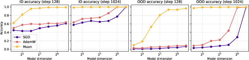
- With one training step, Muon can correctly recover many more of the most frequent facts than SGD.
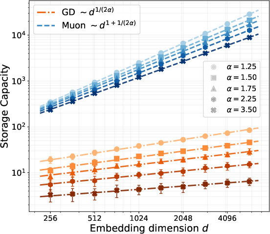
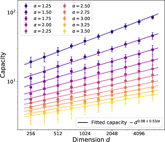
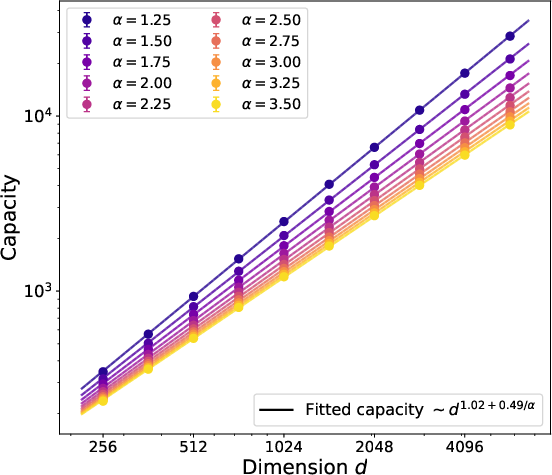
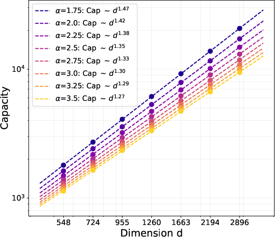
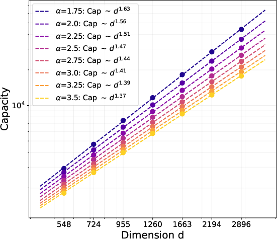
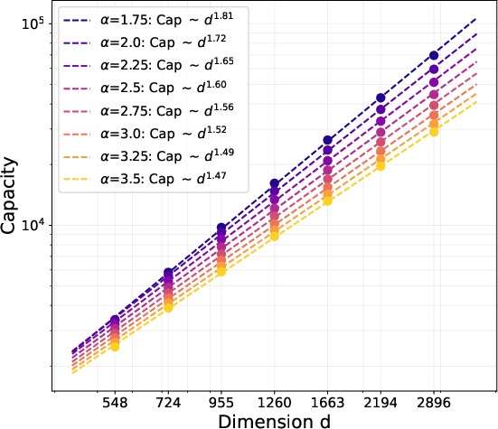
- If the embedding dimension is d and fact popularity follows a power law with exponent α > 1, Muon learns about d1 + 1/(2α) of the top facts, while SGD learns only about d1/(2α). This means Muon’s memory grows much faster with dimension.
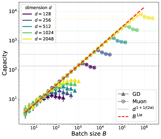
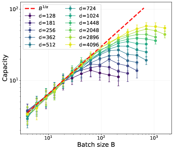
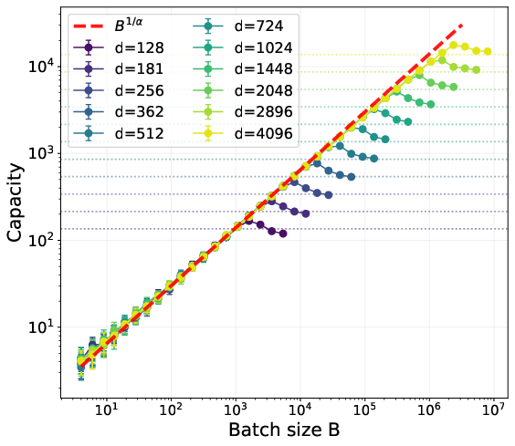
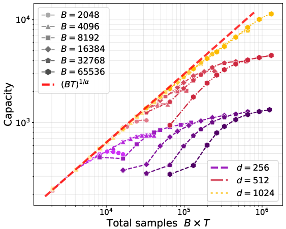
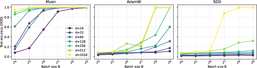
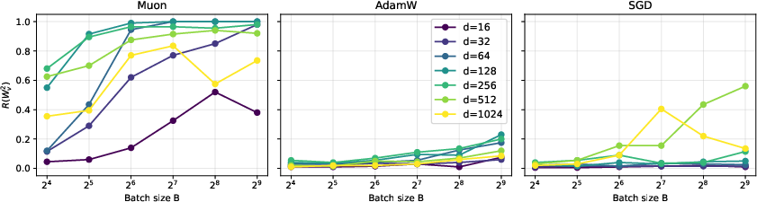
- In minibatches, both methods are limited by how many facts appear in the batch: roughly B1/α. But Muon keeps gaining from bigger batches up to a much larger “critical batch size”—for Muon it’s around dα + 1/2, whereas for SGD it’s about √d. In short, Muon benefits from much larger batches.
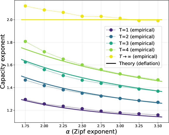
- Multiple-step dynamics:
- Early training: Muon speeds up initial learning a lot—it jumps quickly to storing more than d facts, something SGD cannot do at first.
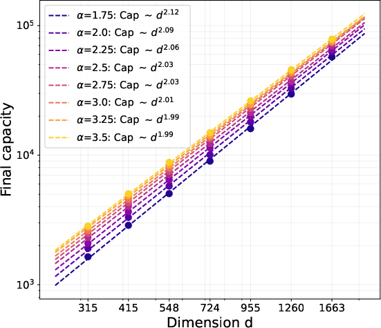
- Later training: As learning progresses, both methods trend toward the best possible limit (roughly d2 facts, the information-theoretic maximum for a d×d matrix). Their long-term speeds become comparable, but Muon’s early acceleration gives it a head start.
- Why this happens:
- With random, overlapping embeddings and power-law frequencies, the gradient has many small directions and a few large ones. Muon boosts the “bulk” of those small directions, helping it pick up many moderately frequent facts at once. SGD mostly follows the largest directions and is slower to capture the rest.
- This “signal amplification” effect explains Muon’s better early performance and its need for larger batches to fully shine.
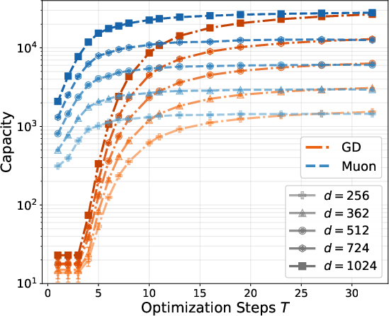
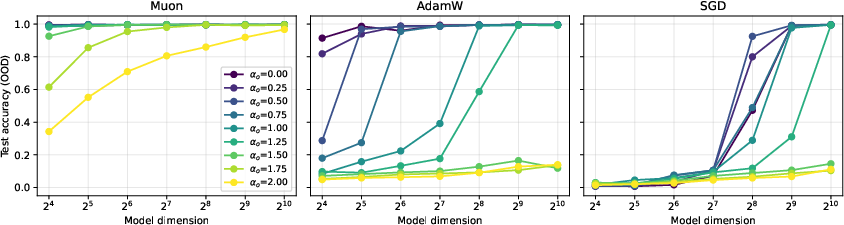
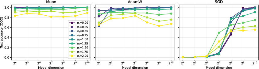
- Experiments:
- Synthetic tests confirm the math: Muon’s capacity scales as predicted and saturates at larger batch sizes than SGD, matching the theory.
Why It Matters
- Practical training insights: For big LLMs, using Muon (or similar spectral methods) can be especially powerful when:
- You have large batch sizes available.
- Your data has a heavy-tailed distribution (common in language).
- You care about fast early learning and storing many facts efficiently.
- Better memory in fewer dimensions: Muon helps models store more features than the embedding dimension by handling superposition well. This is crucial in modern models that must pack huge amounts of knowledge into limited space.
- Guidance for optimizer design and scaling laws: The paper gives a quantitative framework for why spectral updates help and offers scaling rules that can guide training choices, batch sizes, and expectations in more realistic language tasks.
- Big-picture impact: Understanding how and why Muon amplifies useful signals can lead to improved optimizers, better use of large batches, and more efficient memory mechanisms in AI systems, especially for tasks that involve recalling many facts.
Knowledge Gaps
Knowledge gaps, limitations, and open questions
Below is a focused list of what remains missing, uncertain, or unexplored in the paper, phrased to guide concrete follow-up research.
- Robustness to non-Gaussian embeddings: The analysis assumes i.i.d. isotropic Gaussian input/output embeddings. It is unclear how the results change under realistic anisotropic covariances, correlated/tied embeddings (e.g., shared token embeddings), heavy-tailed or structured embeddings, or subspace overlaps.
- Beyond bijective associations: The task assumes a one-to-one mapping (bijection) between inputs and outputs. Many-to-one/one-to-many relations, polysemy, and overlapping associations common in factual knowledge are not analyzed.
- Tied embeddings and self-supervised regimes: The paper assumes separate input and output embeddings; effects of tying (u_i = v_i) or tight correlation (as in language modeling with tied token embeddings) are not derived.
- Applicability beyond linear associative memory: The setting is a single linear matrix W with multiclass logistic loss. Extensions to multi-head attention, nonlinearities (softmax attention, ReLU), residual pathways, and layerwise coupling in transformers remain open.
- Exact Muon vs stabilized Muon: Optimality of the exact polar map (λ → 0) versus the stabilized map h_λ is not rigorously established; the “asymptotic optimality” argument is heuristic and lacks a full proof with anti-concentration and smoothness control.
- Practical Muon implementations: The effect of using a finite number of Newton–Schulz iterations (as done in practice), polynomial approximants h, and finite-precision numerical errors on the predicted scaling laws and batch-size thresholds is not characterized.
- Momentum, weight decay, and other training techniques: The theory “ignores accumulation” and omits momentum, weight decay, gradient clipping, and adaptive learning-rate mechanisms that are standard in large-scale training; their impact on capacity scaling and critical batch size is unknown.
- Multi-step dynamics without thresholding: The multi-step analysis relies on a “thresholded gradient”/deflation heuristic (removing already recovered items). It is open to prove similar scaling laws for the exact cross-entropy dynamics without this approximation.
- Non-asymptotic constants and finite-d behavior: Results are up to polylog factors and for large d, with hidden constants. Explicit, practically relevant finite-sample bounds and constants are not provided.
- Heavier tails and α near/below 1: The theory assumes a power-law frequency with α > 1. Behavior at α ≈ 1 (Zipf-like) or α ≤ 1 is not analyzed, and the exact dependence on α near criticality is unclear.
- Non-stationary or context-dependent frequencies: The analysis assumes a fixed frequency distribution p_i. How nonstationarity, domain shift, curricula, or context-conditioned frequencies affect recovery and batch-size scaling is not addressed.
- Sampling and negative sampling variants: The loss uses a full softmax over all items. How sampled softmax/InfoNCE or other contrastive approximations (common in practice) change signal/noise, capacity, and batch-size thresholds is unknown.
- Cumulative exposure over long horizons: The paper remarks that the (TB){1/α} exposure limit likely governs large T, but does not provide a rigorous derivation for long training horizons or adaptive λ, η schedules.
- Label noise and conflicting facts: Stability of Muon’s signal amplification under mislabeled associations, conflicting entries, or noisy facts is unstudied.
- Initialization effects: All analyses start from W0 = 0. The sensitivity of scaling laws to alternative initializations or warm starts (e.g., pretraining) is not characterized.
- Generality across spectral/matrix optimizers: While the framework mentions a family of spectral maps, rigorous comparisons with other matrix optimizers (e.g., SOAP, Shampoo, Polar-Grad, structure-aware preconditioners) are not provided.
- Optimal λ and η scheduling: The theory prescribes λ and η scalings but does not derive optimal schedules that minimize steps to near d2 capacity under realistic constraints, nor sensitivity to mis-tuning.
- Transition from early acceleration to late-stage convergence: The paper observes Muon’s early advantage and similar asymptotic behavior to SGD. Conditions determining when Muon’s gains persist or vanish across tasks and α, d, B are not fully characterized.
- Capacity near the information-theoretic limit: While multi-step recovery approaches ~d2 (up to logs) for bounded T, a rigorous end-to-end proof of reaching Θ̃(d2) capacity under exact dynamics, finite T and B, and realistic constraints is missing.
- Scale and batch-size trade-offs in practice: The predicted critical batch-size B⋆ for Muon is derived theoretically; a systematic empirical validation across architectures and datasets, and guidance for production training, is not provided.
- Metrics beyond top-1 recovery: Recovery is defined by top-1 argmax. How results change for top-k recall, margin-based criteria, or weighted objectives reflecting heavy-tail utility is unexplored.
- Regularization and implicit bias: The influence of explicit regularizers (weight decay) and implicit biases (e.g., spectral-norm margin maximization) on the learned memory and its generalization is not analyzed.
- N dependence and correlation loss: Some results assume N ≳ d{2α+1} or N = poly(d) and suggest “correlation loss” to relax this, but concrete analyses for small/large N regimes and the precise effect of switching losses are left open.
- Computational costs and stability: Theoretical improvements rely on manipulating spectra of large matrices; the computation/memory overhead, parallelism constraints, and stability considerations at scale are not addressed.
Practical Applications
Immediate Applications
The paper’s results suggest several concrete actions practitioners can take today, especially in settings with heavy‑tailed (Zipf‑like) data and matrix‑valued parameters.
- Large‑batch LLM pretraining: choose spectral optimizers (e.g., Muon) to accelerate early factual recall
- Sector: software/AI (foundation models)
- Use case: In pretraining runs with heavy‑tailed token/fact frequencies, replace SGD/Adam‑style updates with Muon (or a stabilized polar-map approximation) during the early training phase to amplify signal along bulk singular directions and store more associations per step.
- Workflow:
- Start from W0=0 (or early in training), use Muon with a stabilized mapping hλ(z)=z/√(z²+λ²), a small number of Newton–Schulz iterations, and large batch sizes (B≫√d).
- Monitor factual recall (e.g., prompt–response pairs) in early checkpoints; switch to a conventional optimizer later as gradient anisotropy reduces.
- Assumptions/dependencies:
- The benefit is largest when batch sizes are large (SGD saturates near B≈√d, Muon near B≈dα+1/2); data exhibits power‑law frequency α>1; computational budget supports matrix operations for spectral steps; momentum/weight‑decay details may change behavior.
- Throughput and hardware planning: safely increase batch size with Muon to reduce wall‑clock time without early saturation
- Sector: energy/infrastructure and MLOps
- Use case: Because Muon’s critical batch size scales as B*≈dα+1/2 (vs. ≈√d for SGD), distributed training jobs can push batch sizes higher before hitting diminishing returns, improving device utilization and reducing communication overhead.
- Tools: Batch‑size scaling policies in schedulers; cluster‑level auto‑tuning that switches optimizers when B crosses the SGD saturation threshold.
- Assumptions/dependencies: Network bandwidth and memory must support larger batches; the effective “d” (per layer/per head) should be estimated to set B; α must be estimated from data.
- Auto‑tuning of spectral update parameters
- Sector: software/AI tooling
- Use case: Implement an auto‑tuner that estimates the Zipf exponent α (e.g., from token/fact frequency histograms) and sets λ≈d−α (population regime) or λ≈(log d)/B (minibatch regime), and chooses the number of Newton–Schulz iterations to approximate the polar map efficiently.
- Tools/products: A PyTorch/JAX “SpectralStep” module with:
- λ schedule tied to (d, B, α) and per‑layer embedding dimensions
- A fallback to cubic Newton–Schulz when SVD is too costly
- Assumptions/dependencies: Stable numerical implementation of hλ; small extra compute for matrix polynomials; accurate α estimation.
- Faster early performance on heavy‑tailed, imbalanced tasks beyond LLMs
- Sectors: vision (long‑tailed classification), speech, recommender systems
- Use case: For imbalanced datasets with power‑law class distributions, use Muon (or spectral preconditioners) to boost early‑epoch accuracy on head classes and accelerate overall convergence.
- Workflow: Replace or interleave standard optimizer steps with spectral steps during early training; use larger batches for maximal gains.
- Assumptions/dependencies: Matrix‑shaped parameters (e.g., linear/attention layers) and heavy‑tailed label or feature frequencies.
- Knowledge‑injection/fine‑tuning phases emphasizing associative recall
- Sector: software/AI (fine‑tuning, knowledge editing)
- Use case: When adding or reinforcing thousands of “fact” associations (e.g., entity→attribute mappings), employ spectral updates to rapidly increase recall capacity per step.
- Workflow: Aggregate microbatches into large effective batches for Muon; schedule a short Muon phase followed by a standard optimizer for stabilization.
- Assumptions/dependencies: Gains are largest when new facts follow head–tail distributions; sufficient batch accumulation is feasible.
- Lightweight benchmarking of optimizer choices with associative memory tests
- Sector: academia/industry R&D
- Use case: Adopt the paper’s linear associative memory benchmarks (Gaussian embeddings, Zipf frequencies) as a quick, synthetic testbed to compare optimizers’ early‑step capacity and batch‑size saturation before committing to full LLM runs.
- Tools: Open‑source scripts that report “items recovered vs. d and B” and identify the critical batch size per optimizer.
- Assumptions/dependencies: Synthetic tests approximate early training regimes; transfer to non‑linear transformers is empirical.
- Reporting and governance: include optimizer and batch‑size disclosures for fair comparisons and sustainability tracking
- Sector: policy/corporate governance
- Use case: Require reporting of optimizer family (spectral vs non‑spectral), effective batch size, and early‑epoch recall metrics to enable apples‑to‑apples comparisons and estimate energy savings from larger‑B spectral training.
- Dependencies: Organizational policy alignment; standardized metrics for early recall and long‑tail performance.
Long‑Term Applications
As the theory is extended beyond linear associative memory and as tooling matures, the following opportunities become feasible.
- Hybrid optimizers that adaptively orthogonalize bulk singular directions and switch modes over training
- Sector: software/AI
- Use case: Design optimizers that start with spectral norm‑steepest descent (Muon‑like) when gradients are anisotropic and gradually transition to Adam/SGD as isotropy increases, leveraging the paper’s finding that Muon’s advantage is largest early.
- Products: “Hybrid Muon–AdamW” with automatic phase switching based on spectral diagnostics (e.g., singular value spread of layer‑wise gradients).
- Assumptions/dependencies: Reliable online estimation of gradient spectra; additional research on stability with momentum, weight decay, and mixed precision.
- Architecture‑level memory modules exploiting superposition with spectral training
- Sectors: software/AI, robotics (embedded models), mobile/on‑device AI
- Use case: Develop compact associative memory layers (e.g., low‑dimensional key‑value stores) that, trained with spectral updates, store more associations per parameter than standard training—beneficial for edge devices with strict memory budgets.
- Dependencies: Extension of theory to non‑linear layers; hardware support for efficient matrix function approximations.
- Distributed training systems optimized for ultra‑large batch spectral updates
- Sector: energy/infrastructure
- Use case: Build frameworks that maximize throughput under Muon’s larger critical batch size (B*≈dα+1/2), including communication‑efficient implementations of Newton–Schulz and layerwise scheduling.
- Products: Runtime components for pipelining spectral updates; fused kernels for matrix polynomial evaluation.
- Assumptions/dependencies: Stable scaling of spectral methods across thousands of devices; memory footprints manageable; fault tolerance under new compute patterns.
- Long‑tail performance boosters via joint data/optimizer curricula
- Sectors: software/AI, recommender systems
- Use case: Combine spectral early‑phase optimization with sampling curricula that gradually increase exposure to tail items, aiming to improve rare‑item recall without sacrificing head performance.
- Dependencies: Empirical validation in non‑linear models; methods to mitigate interference/forgetting in superposition.
- Knowledge editing and rapid fact updates in deployed LLMs
- Sector: software/AI products
- Use case: Use short spectral update bursts to inject or modify factual associations in specific layers, potentially offering faster and more parameter‑efficient edits than standard fine‑tuning.
- Dependencies: Robust methods to localize updates to relevant layers; safeguards against collateral changes; evaluation for factual consistency.
- Domain‑specific applications with heavy‑tailed distributions
- Healthcare: Clinical NLP often exhibits head–tail distributions (common vs rare conditions). Spectral training could, with further research, improve early acquisition of frequent clinical facts and provide better capacity for rare entities.
- Finance: Document/entity distributions are heavy‑tailed; spectral optimizers may reduce time‑to‑useful performance in domain‑specific pretraining.
- Robotics: Memory‑lean policies storing many state→action associations via superposition in compact matrices trained spectrally.
- Dependencies (all): Safety, validation on non‑linear models; compliance constraints; sensitivity to optimization instabilities.
- Standards and best practices for evaluating associative recall at scale
- Sector: policy/standards bodies, academia
- Use case: Establish benchmarks and reporting guidelines for memory capacity and long‑tail recall under varying batch sizes and optimizers, informed by the paper’s scaling laws.
- Dependencies: Community agreement on metrics; datasets reflecting realistic head–tail distributions.
Notes on assumptions that affect feasibility across applications:
- The paper analyzes a linear associative memory with Gaussian embeddings and a power‑law frequency (α>1); real LLMs are non‑linear, use learned embeddings, and include momentum, regularization, and complex data pipelines.
- Multi‑step results rely on a thresholded‑gradient approximation; exact dynamics in deep networks may differ.
- Spectral steps add computational overhead (SVD or Newton–Schulz); practical benefit depends on efficient approximations and hardware support.
- Mapping “d” to practice typically means per‑head or per‑layer embedding dimensions; α should be estimated from actual data.
- Benefits are most pronounced with large batches; without sufficient B, gains diminish and may not exceed well‑tuned Adam/SGD.
Glossary
- Adam optimizer: An adaptive gradient-based optimization algorithm commonly used to train neural networks, combining momentum and per-parameter learning rate scaling. Example: "the Adam optimizer and its variants"
- Adaptive first-order optimization: A class of gradient-based methods that adapt learning rates using first-order (gradient) information during training. Example: "LLMs with billions of parameters are typically trained using adaptive first-order optimization algorithms."
- Associative memory: A computational model that stores and retrieves input–output associations (facts) so that a query input retrieves its associated output. Example: "the task of learning linear associative memory."
- Bayes optimal (update rule): The decision rule that minimizes expected loss under the data-generating distribution. Example: "The Bayes optimal update rule w.r.t. L is in $\Spec(d)$"
- Bi-orthogonally equivariant: A property of a matrix mapping that commutes with left-right multiplication by orthogonal matrices. Example: "bi-orthogonally equivariant measurable maps"
- Block resolvent integral representation: An analytic representation of matrix functions using block resolvents, useful for series expansions. Example: "we first invoke a block resolvent integral representation amenable to series expansion"
- Cross-entropy loss: A loss function for classification that measures the discrepancy between predicted probabilities and true labels. Example: "and optimizing the cross-entropy loss."
- Critical batch size: The batch size beyond which increasing it does not yield further performance gains. Example: "This further implies that the critical batch size, beyond which increasing batch size does not yield performance gains, is much larger for Muon compared to SGD."
- Daleckii--Krein formula: A formula that provides the Fréchet derivative of matrix functions in terms of spectral data. Example: "The slope can be computed explicitly via the Daleckii--Krein formula"
- Deflation process: Iteratively removing the contribution of already-learned components from updates or gradients. Example: "This can be viewed as a deflation process"
- Haar measure: The unique translation-invariant probability measure on a compact group (e.g., orthogonal group). Example: "averaging $h^{\bU,\bV}$ over Haar measure $\bU,\bV\sim O(d)\times O(d)$"
- Information-theoretic limit: The maximal achievable performance or capacity constrained only by information-theoretic considerations. Example: "both methods eventually converge to the information-theoretic limit at comparable speeds."
- Isotropic Gaussian distribution: A multivariate normal distribution with zero mean and covariance proportional to the identity; directions are equally likely. Example: "drawn i.i.d.~from an isotropic Gaussian distribution"
- Leave-one-out gradient: The gradient computed with one component (e.g., one rank-one term) removed, used for perturbation analysis. Example: "Denote the leave-one-out gradient $\bG_{-i} := \bG -q_iu_iv_i^\top$"
- Logistic regression loss: The loss associated with logistic (softmax) regression, typically cross-entropy over logits. Example: "one step of Muon and SGD on the logistic regression loss under a power law frequency distribution."
- Minibatch: A subset of training examples sampled at each step to compute a stochastic update. Example: "We also consider the minibatch versions of SGD and Muon"
- Moment methods in random matrix theory: Techniques analyzing matrices via moments of their eigenvalue/singular value distributions. Example: "reminiscent of moment methods in random matrix theory."
- Muon: A matrix-based spectral optimizer that updates weights in the direction of the polar factor of the (negative) gradient. Example: "Muon updates each weight matrix in the approximate direction of the polar factor, or spectral orthogonalization, of the negative gradient."
- Newton--Schulz iterations: An iterative scheme to approximate matrix functions (e.g., matrix inverse square root or polar factor) using low-degree polynomials. Example: "one instead approximates $p(\bG)$ via a constant number of Newton--Schulz iterations."
- Polar factor: For a matrix, the unitary/orthogonal factor in its polar decomposition; here, the direction used to precondition updates. Example: "the approximate direction of the polar factor, or spectral orthogonalization"
- Polar map: The mapping that sends a matrix to the orthogonal factor in its polar decomposition. Example: "The polar map is defined as $p(\bG) := \bU\bV^\top$"
- Power-law frequency distribution: A distribution where the probability of an item scales as a negative power of its rank. Example: "the~th item appears with power-law frequency~"
- Singular value decomposition (SVD): A factorization of a matrix into orthogonal factors and nonnegative singular values. Example: "Denote by $\bG = \bU \bS \bV^\top$ the singular value decomposition (SVD) of $\bG$."
- Spectral norm: The largest singular value of a matrix; the operator norm induced by the Euclidean vector norm. Example: "steepest descent with respect to the spectral norm"
- Spectral optimizer: An optimizer that leverages matrix spectra (singular values/vectors) to precondition or modify updates. Example: "matrix-based or spectral optimizers"
- Spectral orthogonalization: Orthogonalizing updates using spectral information (e.g., polar factor) to align steps with principal directions. Example: "polar factor, or spectral orthogonalization"
- Spectrally equivariant: Invariance of an estimator to orthogonal changes of basis; acts diagonally in the singular vector basis. Example: "We first show that the Bayes optimal estimator must be spectrally equivariant"
- Stabilized approximation: A smoothed variant of a matrix function (e.g., polar map) using a stabilizing parameter to control numerical behavior. Example: "we will focus on a stabilized approximation to Muon"
- Stochastic gradient descent (SGD): An optimization method that updates parameters using noisy gradients from minibatches. Example: "Muon versus stochastic gradient descent (SGD)"
- Superposition: Storing many features in overlapping directions so that their number exceeds the ambient dimension. Example: "store items, or features, in superposition"
- Zipf's law: An empirical law in language where word frequency is inversely proportional to its rank. Example: "Motivated by Zipf's law for language modeling"
Collections
Sign up for free to add this paper to one or more collections.