Fusion of Spatio-Temporal and Multi-Scale Frequency Features for Dry Electrodes MI-EEG Decoding
Abstract: Dry-electrode Motor Imagery Electroencephalography (MI-EEG) enables fast, comfortable, real-world Brain Computer Interface by eliminating gels and shortening setup for at-home and wearable use.However, dry recordings pose three main issues: lower Signal-to-Noise Ratio with more baseline drift and sudden transients; weaker and noisier data with poor phase alignment across trials; and bigger variances between sessions. These drawbacks lead to larger data distribution shift, making features less stable for MI-EEG tasks.To address these problems, we introduce STGMFM, a tri-branch framework tailored for dry-electrode MI-EEG, which models complementary spatio-temporal dependencies via dual graph orders, and captures robust envelope dynamics with a multi-scale frequency mixing branch, motivated by the observation that amplitude envelopes are less sensitive to contact variability than instantaneous waveforms. Physiologically meaningful connectivity priors guide learning, and decision-level fusion consolidates a noise-tolerant consensus. On our collected dry-electrode MI-EEG, STGMFM consistently surpasses competitive CNN/Transformer/graph baselines. Codes are available at https://github.com/Tianyi-325/STGMFM.
Paper Prompts
Sign up for free to create and run prompts on this paper using GPT-5.
Top Community Prompts
Explain it Like I'm 14
Explaining “Fusion of Spatio-Temporal and Multi-Scale Frequency Features for Dry Electrodes MI-EEG Decoding”
Overview: What is this paper about?
This paper is about making Brain-Computer Interfaces (BCIs) easier and more comfortable to use in everyday life. BCIs read your brain’s electrical activity (called EEG) and try to understand what you’re thinking or imagining. Here, the authors focus on “motor imagery,” which means imagining moving your hand or foot. They build a new computer model called STGMFM that can better read “dry-electrode” EEG signals—special sensors that don’t need sticky gel—so you can put on a cap quickly and use it at home. Dry electrodes are more comfortable, but their signals are noisier and less stable. The paper shows a way to decode these tricky signals more accurately.
Goals: What questions are they trying to answer?
The paper aims to:
- Improve how well BCIs understand motor imagery from dry-electrode EEG, which is noisier than traditional “wet” electrodes.
- Make the decoding work well across different days (sessions) and different people (subjects), even when the sensor positions and contact quality change.
- Use smart signal features—like the “envelope” of brain rhythms—that stay stable even when the contact is imperfect.
- Combine several “views” of the data so one noisy signal doesn’t ruin the final decision.
Methods: How did they do it?
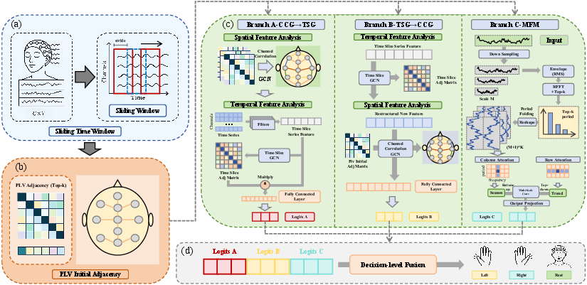
Think of the system like three friendly detectives looking at the same evidence from different angles, then voting on the answer. The model, called STGMFM, has three branches:
- Branch A (Spatial-first, then Time):
- “Spatial” means how EEG channels (sensors) relate to each other. The model first lines up channels that truly work together, using a graph—a map of which sensors are connected.
- Then it looks at how these cleaned-up signals change over time.
- Analogy: First clean and organize microphones around a stadium so the ones picking up the same crowd chant are linked. Then watch how the chant grows or fades during the game.
- Branch B (Time-first, then Spatial):
- First, it stabilizes the signal over time, so quick bursts of noise don’t spread.
- Then it brings together the channels that match well.
- Analogy: First smooth out a shaky video frame-by-frame, then figure out which cameras caught the same scene.
- Branch C (Multi-Scale Frequency Mixer on the Envelope):
- Instead of tracking the exact wiggles of the brain waves (which can be messy), this branch looks at the “envelope”—the outline of how strong the rhythm is at each moment. This is more stable when electrodes don’t touch perfectly.
- It zooms in and out across different time scales to catch both fast rhythms and slow trends.
- Analogy: If a song is hard to hear clearly, listen to how the volume rises and falls over time rather than the exact notes—it’s more reliable.
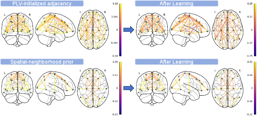
To make the “sensor map” smarter, they start with a brain-inspired trick called PLV (phase-locking value). PLV measures how “in-step” two channels are—like two dancers staying in sync. This helps the model start with a reasonable guess of which sensors are working together, and then it learns small adjustments that fit each person and each day.
The system processes signals in short overlapping windows (like cutting a long recording into small clips), and at the end, the three branches share their opinions. A simple “voting” layer combines them at the decision level, which is more stable than mixing raw features too early.
Training details in simple terms:
- Loss functions and regularization act like rules that prevent the model from “cheating” by memorizing noise.
- A “cosine annealing” schedule slowly reduces the learning rate, like cooling hot metal so it settles into a stable shape.
Results: What did they find and why does it matter?
They recorded dry-electrode EEG from 19 people across two different days, using 23 channels at 250 Hz, for a 3-class motor imagery task. They tested three realistic situations:
- Cross-Session: trained on one day, tested on another day (same person).
- Cross-Subject: trained on some people, tested on a new person.
- Cross-Subject + Fine-tuning: trained on others, then lightly adapted to one session of the new person.
Compared to well-known models (CNNs, Transformers, and graph-based baselines), STGMFM consistently did better:
- Cross-Subject accuracy reached about 57%, higher than others that were mostly around 47–52%.
- With fine-tuning, accuracy climbed close to 60%.
- It also improved other fairness and consistency measures (F1 score, Cohen’s kappa), meaning its predictions were more reliable, not just lucky.
They also ran ablation tests—turning parts on and off—to see what matters:
- Using both graph orders (A and B) helped because they catch different kinds of noise.
- The envelope-based branch (C) added a robust cue when the waveform itself was messy.
- Starting with PLV (the in-step sensor map) and letting it learn small changes reduced mistakes early in training.
- A simple decision-level fusion worked better and more stably than fancier “gated” fusion.
Why this matters: Dry electrodes make BCIs more comfortable and practical for everyday use, but the signals are hard to decode. The new method shows a concrete way to make dry-electrode BCIs work better across days and people, which is key for home rehab, training, and assistive devices.
Implications: What could this lead to?
- More user-friendly BCIs: Faster setup without gel, better comfort, and less need to recalibrate every day.
- Better at-home rehabilitation and training: People could practice motor imagery regularly, with more consistent results across sessions.
- More reliable wearables and assistive tech: Devices can better understand brain signals in everyday environments, even if the cap isn’t perfectly placed.
- Future steps include smarter ways to estimate PLV on the fly, learning how much to trust each branch for each person, and making the model lighter for on-device use.
In short, this paper provides a practical, noise-resistant approach to decoding brain signals from comfortable dry electrodes by combining multiple views—space, time, and stable rhythm envelopes—and carefully fusing their decisions.
Knowledge Gaps
Knowledge gaps, limitations, and open questions
The following list synthesizes what remains missing, uncertain, or unexplored in the paper, framed as concrete items future work can address:
- Dataset accessibility and detailed characterization
- The dry-electrode MI-EEG dataset is not stated as publicly released, limiting reproducibility and external benchmarking; publish the dataset (with metadata) or evaluate on established dry/wet datasets to validate generality.
- SNR, impedance, and artifact profiles of the collected dry recordings are not quantified; include objective measurements (e.g., impedance logs, per-trial SNR, artifact annotations) and correlate them with performance.
- Preprocessing pipeline transparency and robustness
- Critical preprocessing steps (referencing scheme, bandpass/notch filtering, artifact handling such as EOG/EMG removal, normalization) are not described; specify these and evaluate model sensitivity to each step.
- Envelope extraction (e.g., RMS over μ/β) lacks detail on filter design, frequency bands, and windowing; compare alternative band selections and extraction methods (Hilbert, wavelet, short-time Fourier) and report their impact.
- Windowing and time-slice design
- The text describes “overlapping” segments, but experiments use stride equal to window length (non-overlapping); clarify and run sensitivity analyses over window length, stride, and number of slices per trial.
- The choice of 0.5 s slices and nine slices per trial is not justified; ablate slice granularity and placement relative to MI onset to test if performance hinges on specific temporal windows.
- Channel and montage generalization
- Evaluation is limited to one 23-channel dry cap; assess robustness to different montages, fewer/missing channels, and electrode types (e.g., pin vs foam) common in consumer devices.
- The approach assumes a fixed channel set/order; add experiments on channel permutation, dropout, and re-positioning to reflect real-world variability.
- PLV-driven adjacency construction
- PLV computation details (bands, time windows, per-run/per-subject aggregation, Top-k thresholding) are unspecified; document design choices and analyze performance sensitivity to PLV parameters.
- Only PLV is explored; compare against other connectivity metrics (coherence, imaginary coherence, wPLI, mutual information) to determine the most robust prior under dry-electrode noise.
- Graph learnability is constrained only by L1; investigate symmetry, nonnegativity, and stability constraints (e.g., Laplacian regularization) to preserve physiological interpretability while adapting to sessions.
- No analysis of how learned adjacencies vary across subjects/sessions; quantify consistency and physiologic plausibility of the adapted graphs (e.g., edge patterns in sensorimotor areas).
- Time-slice graph (TSG) design and causality
- The TSG adjacency is learned without explicit temporal structure; explore directed, lagged, or kernel-based edges to encode causality and time-order constraints.
- Initialization and regularization of TSG are not detailed; ablate different initializations (identity, chain, local temporal neighborhoods) and penalties to balance fit vs overfitting.
- Multi-Scale Frequency Mixer (MFM) branch specification
- The “Top-1 dominant period” choice is heuristic; compare Top-k period selection, multi-band envelopes, and alternative multi-resolution tokenization (wavelet scalograms, synchrosqueezing).
- The imaging–decoupling–mixing pipeline lacks formal specification; provide algorithmic details (image size, axes definitions, mixing operations) and complexity estimates, then test sensitivity to each component.
- Claims of ERD/ERS alignment are not validated; add objective interpretability analyses (e.g., per-class μ/β ERD time courses, channel-wise contributions) to confirm neurophysiological alignment.
- Fusion strategy and potential implementation inconsistency
- Decision fusion uses a simple linear head, but equation “hat y = argmax_k z_A” suggests predicting from a single branch; clarify and correct this to “argmax over fused logits,” and compare against stronger stacking (logistic regression, calibrated averaging) and per-subject adaptive fusion.
- Explore feature-level fusion and attention-based fusion under strict regularization to assess whether decision-level fusion is optimal in low-sample regimes.
- Baselines and significance testing
- Classical pipelines (FBCSP, Riemannian geometry) are not included as baselines; add them to contextualize gains under dry conditions.
- Statistical significance of improvements (paired tests, effect sizes) is not reported; provide subject-wise statistics and confidence intervals to substantiate robustness claims.
- Robustness to artifacts and non-stationarity
- No stress tests on artifact robustness (simulated contact loss, motion, EMG/EOG contamination); design controlled perturbations and report degradation curves.
- The graphs are static per trial; investigate dynamic graphs that evolve within trials to model non-stationarity typical of dry EEG.
- Cross-condition and cross-domain generalization
- Generalization is tested across sessions/subjects within one dataset; evaluate cross-hardware, cross-lab, and wet-to-dry transfer to quantify domain shift resilience.
- The task is three-class MI; test scalability to more classes and hybrid paradigms (e.g., MI+SSSEP) to assess broader applicability.
- Data efficiency, adaptation, and augmentation
- Despite trial scarcity, no data augmentation (noise injection, time warping, frequency perturbation), semi/self-supervised pretraining, or test-time adaptation is explored; benchmark these strategies to reduce calibration time.
- Fine-tuning protocol details (number of target-session trials, calibration duration) are absent; quantify the minimal supervision needed for acceptable performance.
- Efficiency and deployment constraints
- Model size, FLOPs, memory footprint, and inference latency on edge hardware are not reported; provide efficiency metrics and compare with on-device constraints typical for wearable BCIs.
- Channel pruning and architecture slimming are mentioned as future work but not studied; systematically evaluate pruning strategies and their accuracy–efficiency trade-offs.
- Interpretability and error analysis
- Beyond adjacency visualization, there is limited interpretability; add channel-wise saliency, scalp maps, and failure-case analyses to understand misclassifications and inform model trust.
- Per-class confusion patterns and their relation to neurophysiological signatures are not analyzed; include confusion matrices and class-specific feature inspections.
- Experimental protocol details
- Trial structure (cue timing, MI onset/offset, rest periods) is not described; document timing to allow replication and to interpret learned temporal dependencies.
- Class balance and random seed control are not specified; ensure balanced sampling and report multiple seeds to assess stability.
- Theoretical framing and guarantees
- There is no theoretical analysis of why dual-order graph propagation hedges noise or when it may fail; formalize conditions under which CCG→TSG vs TSG→CCG excels, and derive bounds or diagnostic criteria to select branch dominance per subject/session.
Practical Applications
Overview
This paper proposes STGMFM, a tri-branch decoding framework tailored to dry-electrode motor imagery (MI) EEG. It fuses complementary spatio-temporal graph processing (channel-correlation graph CCG and time-slice graph TSG in dual orders) with a lightweight Multi-Scale Frequency Mixer (MFM) operating on amplitude envelopes (ERD/ERS). PLV-initialized connectivity priors stabilize learning under low SNR and contact variability typical of dry EEG. Across cross-session and cross-subject protocols, STGMFM outperforms strong CNN/Transformer/GCN baselines and reduces dependence on extensive calibration.
Below are practical real-world applications derived from the paper’s findings, methods, and innovations. Each item states sectors, potential tools/products/workflows, and assumptions/dependencies.
Immediate Applications
The following applications can be deployed now or with minimal engineering, leveraging the released code and the model’s robustness to dry-EEG noise and cross-session drift.
- Dry-EEG MI-BCI decoder for assistive control in home rehab and clinics (Sectors: healthcare, robotics; Tools/Workflows: integrate STGMFM as the decoding engine in existing BCI software/firmware; use the paper’s “cross-subject pretrain + single-session fine-tuning” to cut onboarding time; decision-level fusion and envelope branch for noise tolerance; Assumptions/Dependencies: access to multi-channel dry caps ~23 channels with consistent montage; basic artifact handling; clinician supervision for safety-critical tasks).
- Calibration-lite onboarding for commercial dry-EEG systems (Sectors: consumer/wearable BCI; Tools/Workflows: ship devices with a pre-trained STGMFM model and run a short single-session fine-tune; sliding-window inference; Assumptions/Dependencies: brief calibration session (e.g., 5–10 minutes) to reach stable accuracy; consistent electrode placement across sessions; clear task instructions for MI).
- Smart-home control for motor-impaired users (Sectors: daily life, smart home; Tools/Workflows: map MI classes to commands (lights, TV, curtains) using STGMFM real-time inference; safety gating via decision-level fusion and confidence thresholds; Assumptions/Dependencies: reliable Wi-Fi/home hub integration; user training; safeguards against false positives and fatigue).
- At-home neurofeedback for MI training (Sectors: healthcare, education; Tools/Workflows: visualize envelope-based ERD/ERS patterns (MFM branch) for feedback; progressive training curricula; Assumptions/Dependencies: clear visualization UI; band selection (mu/beta); clinician or therapist remote oversight for protocol adherence).
- Retrofitting existing MI decoders with PLV-initialized graphs (Sectors: software/BCI R&D; Tools/Workflows: add PLV-based adjacency initialization to existing GNN/GCN pipelines to stabilize spatial relations under dry-electrode variability; Assumptions/Dependencies: stable phase estimation per trial; appropriate top-k sparsification and normalization).
- Noise-robust preprocessing plugin using envelope dynamics (Sectors: software; Tools/Workflows: extract amplitude envelopes and apply multi-scale mixing (MFM) as a module before downstream classifiers; Assumptions/Dependencies: bandpass filtering to alpha/mu/beta; parameterization of multi-resolution imaging and mixing; compatibility with current pipelines).
- Academic benchmarking and replication with open-source code (Sectors: academia; Tools/Workflows: adopt the GitHub implementation for dry-EEG baselines; reproduce cross-session and cross-subject protocols; run ablations to compare PLV priors, dual graph orders, and fusion schemes; Assumptions/Dependencies: dataset availability with dry electrodes; adherence to the paper’s windowing and training recipe).
- Edge-friendly inference profiles for embedded devices (Sectors: software/hardware; Tools/Workflows: deploy the lightweight MFM branch and decision-level fusion on SBCs or mobile GPUs for near-real-time control; Assumptions/Dependencies: latency targets (e.g., <250 ms), memory constraints; potential pruning/quantization to fit device budgets).
Long-Term Applications
These applications require further research, scaling, validation, or engineering (e.g., larger datasets, regulatory approval, hardware co-design).
- Medical-grade dry-EEG BCI for mobility, communication, and prosthetics (Sectors: healthcare, robotics; Tools/Products: integrated wheelchair/exoskeleton/prosthetic controllers powered by STGMFM; workflows for cross-session drift mitigation and rapid personalization; Assumptions/Dependencies: stringent clinical validation; regulatory clearance; robust performance beyond ~60% 3-class accuracy reported; fail-safe design).
- AR/VR control via wearable dry-EEG headsets (Sectors: consumer, software; Tools/Products: hands-free interaction in XR using MI classes; Assumptions/Dependencies: ergonomic, high-density dry caps with stable impedance; minimization of motion artifacts; UX for training and feedback).
- Federated learning personalization across users and sessions (Sectors: software, privacy; Tools/Workflows: subject-aware fusion layers and adaptive PLV estimation trained via federated protocols; Assumptions/Dependencies: privacy-compliant data governance; cross-device synchronization; robustness to non-IID distributions).
- Channel pruning and hardware co-design for ultra-low-power edge BCI (Sectors: hardware, energy; Tools/Products: pruned STGMFM variants on custom SoCs/ASICs; Assumptions/Dependencies: co-optimization of accuracy vs. power; on-head thermal constraints; standardized electrode layouts).
- Multi-modal fusion (EEG+EMG/EOG/IMU) to reduce false positives (Sectors: healthcare, robotics; Tools/Workflows: augment STGMFM with sensor fusion to disambiguate MI from artifacts; Assumptions/Dependencies: synchronized multi-sensor acquisition; sensor placement; fusion training).
- Standardization of dry-EEG BCI evaluation protocols (Sectors: policy, healthcare; Tools/Workflows: formalize cross-session and cross-subject benchmarks, metrics (ACC, kappa, F1) and calibration procedures; Assumptions/Dependencies: consensus through standards bodies (IEEE/ISO), multi-site studies, public datasets).
- Insurance reimbursement for home-based neurorehab BCIs (Sectors: policy, healthcare; Tools/Workflows: clinical outcome studies demonstrating functional gains with MI training aided by STGMFM; Assumptions/Dependencies: high-quality RCTs; cost-effectiveness analyses; clinician training).
- Safety-critical BCI interfaces for smart home and vehicle control (Sectors: policy, consumer/automotive; Tools/Workflows: multi-level confirmation, lockouts, and explainability (confidence/consensus indicators from fusion); Assumptions/Dependencies: cybersecurity, liability frameworks, human factors validation).
- Large-scale dry-EEG datasets and foundation models (Sectors: academia; Tools/Workflows: collect and share diverse dry-EEG MI recordings to pretrain domain-general models; Assumptions/Dependencies: privacy, consent, harmonized hardware/montages; data curation and bias mitigation).
- Clinical decision support using connectivity maps (Sectors: healthcare; Tools/Products: PLV-based connectivity dashboards to guide electrode placement and assess MI readiness or training progress; Assumptions/Dependencies: validated correlates between PLV patterns and functional outcomes; clinician-facing visualization tools).
Notes on feasibility across applications:
- Reported performance (e.g., ~57% cross-subject accuracy and ~60% with single-session fine-tuning on a 3-class task) is promising but may be insufficient for high-stakes control; applications should include safeguards, multi-modal redundancy, and user training.
- Robust deployment depends on consistent electrode montage, impedance management, and artifact mitigation; comfort and stability of dry caps are critical.
- Real-time constraints are achievable with lightweight branches and potential model pruning/quantization, but power and latency budgets must be validated on target hardware.
- Regulatory, privacy, and ethical considerations (especially for clinical and safety-critical use) require additional evidence, standardization, and compliance work.
Glossary
- AdamW: An optimizer that decouples weight decay from the gradient update in Adam to improve generalization; "We train 1000 epochs with AdamW (initial learning rate ), batch size 32, dropout 0.2, cosine-annealing schedule, and L1/L2 regularization on graph weights and classifier."
- amplitude envelope (RMS): A smooth measure of signal magnitude over time, often computed via root-mean-square, emphasizing slow modulations over instantaneous phase; "The third branch operates on the amplitude envelope (RMS) (e.g., band), which makes ERD/ERS modulation explicit and phase-invariant."
- analytic phase: The instantaneous phase of a signal derived from its analytic representation (e.g., via the Hilbert transform); "For channels and with analytic phases and ,"
- bandpower: The power of a signal within a specific frequency band, used to characterize EEG rhythms; "Classical MI pipelines relied on Common Spatial Pattern/bandpower and linear classifiers or Riemannian geometry on covariances"
- Brain–Computer Interface (BCI): A system that translates brain activity into commands for external devices or software; "Non-invasive Electroencephalography (EEG) is the most accessible neural sensing modality for daily-life Brain Computer Interface (BCI) applications."
- channel-correlation graph (CCG): A graph where nodes are EEG channels and edges encode inter-channel relationships or correlations; "Branches A/B pair a channel-correlation graph (CCG) and a time-slice graph (TSG) in opposite orders (CCGTSG vs.\ TSGCCG),"
- Cohen's kappa: A metric that measures classification agreement adjusted for chance; "We report Accuracy (ACC), Cohen's kappa, and F1."
- Common Spatial Pattern (CSP): A spatial filtering method that maximizes variance differences between classes in EEG; "Classical MI pipelines relied on Common Spatial Pattern/bandpower and linear classifiers or Riemannian geometry on covariances"
- cosine annealing: A learning-rate schedule that follows a cosine curve to promote smoother convergence; "Cosine-annealed learning rates promote smooth convergence and better generalization."
- cross-entropy: A classification loss measuring the divergence between predicted probabilities and true labels; "We train with cross-entropy"
- decision-level fusion: Combining predictions (e.g., logits) from multiple branches/models to form a final decision; "Physiologically meaningful connectivity priors guide learning, and decision-level fusion consolidates a noise-tolerant consensus."
- degree-normalization: Scaling the adjacency matrix by node degrees (e.g., ) to stabilize graph propagation; "symmetrize, and degree-normalize to obtain $\tilde{\mathbf{A}=\mathbf{D}^{-1/2}\mathbf{A}\mathbf{D}^{-1/2}$."
- depthwise–pointwise 1D convolution: A factorized convolution that applies per-channel (depthwise) filters followed by 1×1 (pointwise) mixing, improving efficiency; "shared temporal convolutional block (depthwise–pointwise $1$D convolution with GELU/normalization)"
- ERD/ERS: Event-related desynchronization/synchronization, reflecting decreases/increases in power of EEG rhythms during tasks; "aligned with ERD/ERS to offer a robust temporal cue when instantaneous waveform detail is unreliable."
- functional connectivity: Statistical relationships (e.g., synchrony) between signals reflecting coordinated neural activity; "To encode functional connectivity as a prior, we build an initial adjacency from the phase-locking value (PLV)."
- GELU: Gaussian Error Linear Unit, an activation function blending linear and nonlinear behavior; "shared temporal convolutional block (depthwise–pointwise $1$D convolution with GELU/normalization)"
- global average pooling (GAP): A pooling operation that averages features over an entire spatial/temporal dimension; "A global average pooling (GAP) and a linear head yield ."
- graph neural network (GNN): Neural architectures designed to operate on graph-structured data; "Electroencephalography, motor imagery, dry electrodes, graph neural network, frequency mixing"
- graph propagation: The process of spreading and transforming node features via the graph adjacency in a layer; "Branch A first performs graph propagation on the channel graph to align truly cooperating electrodes and suppress mismatched ones."
- impedance: The opposition to electrical current at the skin–electrode interface, affecting signal quality; "the unstable skinâelectrode coupling often elevates and fluctuates impedance, lowering Signal-to-Noise (SNR) and amplifying motion/contact artifacts"
- inductive bias: Assumptions built into a model’s architecture that guide learning preferences; "We insert a lightweight shared temporal block between CCG and TSG to align feature spaces and add local temporal expressiveness without disturbing the graph inductive bias."
- inter-subject variability: Differences in signal characteristics across different participants; "What is more, inter-subject variability is exacerbated due to hair and pressure differences."
- L1 regularization: A sparsity-promoting penalty using the ℓ1 norm to reduce overfitting; "We train with cross-entropy and combine sparsity on graph-increment parameters with weight decay (AdamW)."
- L2 regularization: A weight-decay penalty using the ℓ2 norm to improve generalization; "We train with cross-entropy and combine sparsity on graph-increment parameters with weight decay (AdamW)."
- logits: The raw, unnormalized scores output by a classifier before applying softmax; "Each branch outputs logits, and a shallow head fuses them at the decision level,"
- motor imagery (MI): The mental simulation of movement used to elicit characteristic EEG patterns; "Currently, most existing Motor Imagery (MI) decoders were designed/validated under wet-electrode assumptions,"
- Multi-Scale Frequency Mixer (MFM): A module that aggregates information across multiple frequency scales to capture robust envelope dynamics; "We introduce a lightweight Multi-Scale Frequency Mixer that extracts phase-invariant, multi-scale temporal cues aligned with ERD/ERS."
- μ/β band: EEG frequency ranges (mu: ~8–13 Hz, beta: ~13–30 Hz) associated with motor processes; "The third branch operates on the amplitude envelope (RMS) (e.g., band), which makes ERD/ERS modulation explicit and phase-invariant."
- phase synchrony: The alignment of phases between signals indicating coordinated activity; "Connectivity priors such as PLV provide phase-synchrony graphs that are amplitude-invariant and physiologically meaningful"
- phase-locking value (PLV): A measure of phase synchrony reflecting the consistency of phase differences across time; "To encode functional connectivity as a prior, we build an initial adjacency from the phase-locking value (PLV)."
- rfft: The real-input fast Fourier transform used to compute spectral components efficiently; "by selecting dominant periods/frequencies (rfft) and mapping the $1$D signal to a compact timeâfrequency lattice."
- Riemannian geometry: Geometry on curved spaces (e.g., SPD covariance manifolds) used for more natural comparisons of covariance matrices; "Classical MI pipelines relied on Common Spatial Pattern/bandpower and linear classifiers or Riemannian geometry on covariances"
- Signal-to-Noise Ratio (SNR): The ratio of signal power to noise power indicating recording quality; "Dry recordings pose three main issues: lower Signal-to-Noise Ratio with more baseline drift and sudden transients;"
- time–frequency lattice: A compact grid representation of signal content across time and frequency; "and mapping the $1$D signal to a compact timeâfrequency lattice."
- time-slice graph (TSG): A graph whose nodes are temporal windows (slices) of a signal, modeling inter-slice dependencies; "Branches A/B pair a channel-correlation graph (CCG) and a time-slice graph (TSG) in opposite orders (CCGTSG vs.\ TSGCCG),"
- TimeMixer: A multiscale time-series model that mixes information across learned periods; "recent âmixersââ learn multi-period structure with compact, multi-resolution tokenization, including TimeMixer and its successor TimeMixer++ by Wang et al."
- Top-k sparsification: Keeping only the k strongest connections per row/column to make a graph sparse; "We remove self-loops, sparsify by per-row Top- (or a threshold), symmetrize, and degree-normalize to obtain $\tilde{\mathbf{A}=\mathbf{D}^{-1/2}\mathbf{A}\mathbf{D}^{-1/2}$."
Collections
Sign up for free to add this paper to one or more collections.

