A Scalable Measure of Loss Landscape Curvature for Analyzing the Training Dynamics of LLMs
Abstract: Understanding the curvature evolution of the loss landscape is fundamental to analyzing the training dynamics of neural networks. The most commonly studied measure, Hessian sharpness ($λ_{\max}H$) -- the largest eigenvalue of the loss Hessian -- determines local training stability and interacts with the learning rate throughout training. Despite its significance in analyzing training dynamics, direct measurement of Hessian sharpness remains prohibitive for LLMs due to high computational cost. We analyze $\textit{critical sharpness}$ ($λ_c$), a computationally efficient measure requiring fewer than $10$ forward passes given the update direction $Δ\mathbfθ$. Critically, this measure captures well-documented Hessian sharpness phenomena, including progressive sharpening and Edge of Stability. Using this measure, we provide the first demonstration of these sharpness phenomena at scale, up to $7$B parameters, spanning both pre-training and mid-training of OLMo-2 models. We further introduce $\textit{relative critical sharpness}$ ($λ_c{1\to 2}$), which quantifies the curvature of one loss landscape while optimizing another, to analyze the transition from pre-training to fine-tuning and guide data mixing strategies. Critical sharpness provides practitioners with a practical tool for diagnosing curvature dynamics and informing data composition choices at scale. More broadly, our work shows that scalable curvature measures can provide actionable insights for large-scale training.
Paper Prompts
Sign up for free to create and run prompts on this paper using GPT-5.
Top Community Prompts
Explain it Like I'm 14
Overview
This paper is about understanding how “steep” or “bumpy” the training landscape of LLMs is, and how that affects training. The authors introduce a new, fast way to measure how steep the landscape is around the model during training. This lets them track important training behaviors in very big models (up to 7 billion parameters) that were previously too expensive to measure.
What is the paper trying to figure out?
In simple terms, the paper asks:
- How can we measure how risky it is to take a bigger step during training without making the model worse?
- Can a fast measurement capture the same training patterns we see with slow, fancy methods?
- Do these patterns hold for very large models in real training, not just tiny test setups?
- Can this measurement help us fine-tune models without forgetting what they learned before?
How did they study it? (Methods in everyday language)
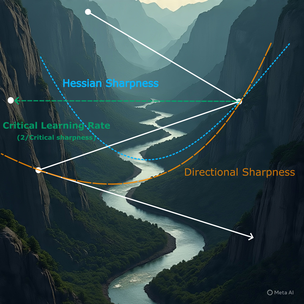
Think of training a model like hiking in a huge landscape of hills and valleys. The “loss” is your height: lower is better. The shape of the land around you (how steep it gets in different directions) affects how big a step you can safely take without climbing back up.
- Traditional measure (Hessian sharpness): This looks for the steepest nearby slope in any direction. It’s very precise but extremely slow and hard to compute for giant models.
- Their new measure (critical sharpness): Instead of checking every direction, they do something simpler and much faster.
- They look at the direction the optimizer already wants to step (the “update direction”).
- They test different step sizes in that one direction to find the biggest step that still goes down the hill (loss gets better). If they step too far, the loss goes up.
- The “critical learning rate” is the step size where going any bigger starts to make things worse.
- “Critical sharpness” is just a way of turning that step size into a number for “how steep it is” in that direction. Bigger sharpness means a smaller safe step.
This is like edging forward toward a cliff: you carefully test how far you can go before it gets dangerous. The key win is speed: they only need a handful of quick “forward passes” (running the model to compute loss) to find this safe limit, instead of doing heavy second-derivative math.
They also define “relative critical sharpness”: when fine-tuning on a new task, you measure how far you can step in the new-task direction before performance on the original task gets worse. This helps you see if you’re leaving the “pre-training basin” (the safe valley the model originally sat in).
What did they find, and why does it matter?
The authors confirm several important training patterns, now at large scale:
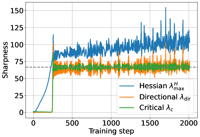
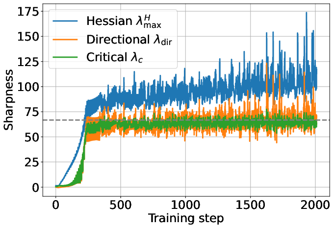
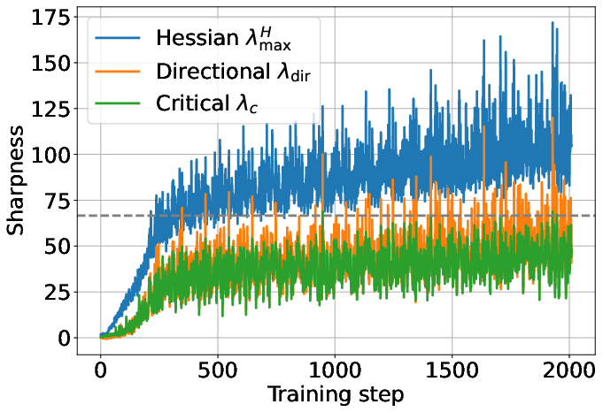
- Progressive sharpening: As training goes on, the landscape around the model tends to get steeper. That means the safe step size naturally shrinks over time.
- Edge of Stability: Models often train right at the boundary where steps are as large as possible without making things worse. With their fast measure, they can see the model “hover” near that edge during training.
- Works at scale: These patterns aren’t just for small toy models. They show them in real LLM training up to 7B parameters (OLMo-2), both during pre-training and mid-training.
- Practical for fine-tuning and avoiding forgetting: Using relative critical sharpness, they study mixing old (pre-training) data with new (specialized) data during fine-tuning. They show:
- If you mostly train on new data (like math), you may “leave the pre-training basin,” improving math skills but risking drops on general knowledge tasks.
- If you keep enough pre-training data in the mix, you stay in the basin and better preserve general abilities.
- There’s a “sweet spot” in the mix where you can push math while keeping general skills. In their tests, this was around 60–70% pre-training data in the mix.
- Task-specific trade-offs:
- GSM8K (math reasoning) improved more when stepping outside the pre-training basin.
- MMLU (broad knowledge and reasoning) did better when staying inside the basin.
- Their measurement helps pick the right data mix and learning rate to match your goal.
Why this matters: Critical sharpness is fast, simple to compute, and tracks the same big behaviors as the expensive method. It gives training teams a practical tool to detect instability, tune learning rates, and design data mixes at LLM scale.
What could this change going forward? (Implications)
- Better monitoring and safer training: Teams can quickly spot when they’re near the “too-big step” zone and adjust learning rates or schedules before training goes off track.
- Smarter fine-tuning: Relative critical sharpness helps choose how much old vs. new data to mix so the model learns new skills without forgetting old ones. It reveals when you’re about to leave the pre-training basin and what that means for different benchmarks.
- Scalable insights: Because it needs only a few forward passes, this method works on giant models where older, precise methods are simply impractical.
Overall, the paper shows that a simple, scalable measure can reveal important training dynamics in large models and guide real decisions—like learning-rate choices and data composition—without heavy computation.
Knowledge Gaps
Knowledge gaps, limitations, and open questions
Below is a concise list of missing pieces and unresolved questions that, if addressed, could make the proposed curvature measures more robust, general, and actionable at scale:
- Quantify the discrepancy between critical sharpness () and Hessian sharpness () in large models: how large can the gap get in practice, and under what alignment conditions does hold for LLMs?
- Establish statistical reliability of the critical learning rate () under stochastic mini-batch noise: sensitivity to batch size, batch reuse vs. held-out batches, and variance/confidence intervals for estimates.
- Specify a standardized evaluation protocol for during line search (same training batch vs. fresh batch vs. validation set) and quantify the bias each choice introduces.
- Characterize the overhead of measuring at LLM scale (compute, latency, memory, weight swaps) and provide guidance on measurement cadence (how often) to balance fidelity vs. cost.
- Test robustness of the line-search assumptions: non-monotonic loss along the line, rugged local landscapes, and step sizes outside the local quadratic regime; add safeguards if the loss is not unimodal along .
- Incorporate optimizer momentum explicitly: the line search uses the current update direction , but Adam/AdamW’s momentum and EMA alter the effective next-step direction; analyze and correct for this mismatch.
- Extend the AdamW stability threshold analysis to include the role of and practical details of decoupled weight decay; validate the theoretical thresholds empirically across a grid of , , and decay strengths.
- Analyze interactions with gradient clipping and mixed-precision/dynamic loss scaling, which are ubiquitous in LLM training and could mask or distort edge-of-stability signals.
- Assess generality across optimizers beyond AdamW (e.g., Adafactor, SGD with momentum, Lion) and propose optimizer-specific formulations of with validated thresholds.
- Evaluate architectural dependence: normalization (RMSNorm vs. LayerNorm), activation functions, positional encodings, Mixture-of-Experts, parameter sharing—does retain its diagnostic value across these variants?
- Scale beyond 7B: do progressive sharpening and the proposed thresholds persist at tens of billions of parameters and with larger context windows?
- Provide direct large-scale validation against Hessian-based proxies (e.g., top HVP via subsampled or blockwise methods) to empirically bound the error of as a curvature proxy in LLMs.
- Compare to alternative curvature measures (empirical Fisher/GGN, Hessian trace, SAM sharpness, gradient norms) in predicting instabilities, EoS behavior, and downstream generalization at scale.
- Determine whether online learning-rate control driven by (e.g., staying at the edge) improves training speed/stability vs. standard warmup/decay schedules for LLMs.
- Examine batch-size effects on in LLM training (the paper shows small-scale trends only): derive or fit scaling laws linking batch size, noise scale, and critical sharpness.
- Develop per-layer or block-wise critical sharpness diagnostics to inform layer-wise learning-rate schedules or targeted regularization.
- Clarify inclusion/exclusion of weight decay in the measured update direction during line search; quantify how decoupled decay alters estimates and EoS thresholds.
- Engineering detail: specify safe, reproducible implementations for large-scale distributed setups (parameter swaps, optimizer-state isolation, avoiding side effects) and release code to reduce integration risk.
- For the “pre-trained basin” concept, provide a formal geometric/operational definition and empirical basin-membership tests (beyond the one-step proxy) over multi-step finetuning trajectories.
- Validate the predictive power of initial for long-horizon forgetting: does a safe initial region remain safe after many updates, or does the boundary drift rapidly?
- Extend relative critical sharpness to multi-objective training (more than two losses) and design an algorithm to adapt data mixing ratios online based on a vector of measurements.
- Generalize beyond math finetuning: test whether the “sweet spot” prediction holds for other domains (code, safety/harms, multilingual, RLHF) and for parameter-efficient finetuning (LoRA/QLoRA), where is low-rank.
- Investigate long-context effects: does measured on short contexts predict stability and forgetting for long-context tasks, or is a context-aware measurement necessary?
- Study whether (or its trends) correlates with out-of-distribution robustness and generalization across checkpoints, clarifying the mixed literature on sharpness and generalization.
- Identify early-warning thresholds using that anticipate catastrophic loss spikes or divergence events in large-scale runs, and test their precision/recall.
- Explore how quickly changes under distribution shift or data-mixture changes; propose measurement schedules and smoothing strategies for non-stationary training.
- Analyze failure modes where critical learning rates greatly exceed due to gradient–eigenvector misalignment; characterize regimes and propose corrections or confidence bands.
Practical Applications
Immediate Applications
The following applications can be deployed now using the paper’s forward-pass-only estimation of critical sharpness (λc) and relative critical sharpness (λc1→2), with minimal changes to existing large-scale training pipelines.
- Real-time stability monitoring and alerting in LLM training (software/ML infrastructure)
- Use λc to track progressive sharpening and Edge of Stability (EoS) during training runs; trigger alerts or automatic interventions when the current learning rate exceeds the stability threshold implied by λc.
- Tools/products/workflows: Training-dashboard integrations (W&B, TensorBoard, MLflow) that log λc over time; on-call runbooks that reduce LR or adjust weight decay when λc drops.
- Assumptions/dependencies: Access to the optimizer’s current update direction and ability to perform a handful of forward passes on the same batch; modest wall-clock overhead (~5–6 forward passes per measurement).
- Automated learning-rate warmup calibration (software/ML infrastructure)
- Replace ad-hoc warmup with λc-informed initialization: pick the initial LR so that η0 ≈ κ * 2/λc (with κ < 1 as a safety factor), then ramp into the stable regime quickly without instability.
- Tools/products/workflows: LR schedulers that query λc at a few early steps to set warmup peak; plug-ins for PyTorch/DeepSpeed/Lightning.
- Assumptions/dependencies: λc estimation remains stable for early steps; single-batch representativeness for LR selection.
- Stable-phase LR ceiling enforcement (software/ML infrastructure)
- Keep training near—but safely inside—the EoS by capping η ≤ α * 2/λc (α ≤ 1), preventing loss spikes and divergence without costly Hessian-vector products.
- Tools/products/workflows: “Edge-aware” LR controllers that periodically probe λc and set per-phase caps.
- Assumptions/dependencies: Measurements at a sub-sampled cadence (e.g., every N steps) are sufficient; LR updates do not conflict with optimizer internals (momentum states).
- Data-mix selection to mitigate catastrophic forgetting in finetuning (industry applied research; healthcare, finance, software)
- Use relative λc1→2 (pretrain loss L1 versus finetune update direction on L2) to choose how much pretraining data to include in a finetune mix so the update stays inside the “pretrained basin” when desired; balance task specialization (e.g., math) vs. general reasoning (e.g., MMLU).
- Tools/products/workflows: A “mix tuner” that sweeps a few candidate pretrain ratios, measures λc1→2 across target benchmarks, and recommends a ratio and LR; applies to domain-specific finetuning (EHR for healthcare, filings for finance).
- Assumptions/dependencies: Access to pretraining-like data slices for rehearsal; relative λc correlates with evaluation metrics in the target setting (validated at 7B OLMo-2, may vary by model/data).
- Continual-learning rehearsal budgeting (academia and applied ML)
- During task sequences, set rehearsal fraction dynamically so η stays below the λc1→2 boundary for important prior tasks, preventing rapid forgetting.
- Tools/products/workflows: Curriculum schedulers that monitor relative λc to previous tasks and adjust rehearsal sampling on-the-fly.
- Assumptions/dependencies: Reasonable proxy batches for all “protected” tasks; storage or on-demand access to rehearsal data.
- RLHF and multi-objective finetuning guardrails (alignment, safety, software)
- Compute λc1→2 to keep RLHF or preference-optimization updates from leaving the pretraining basin too abruptly; gate PPO/learning-rate increases when pretraining loss is predicted to rise.
- Tools/products/workflows: Alignment pipelines that periodically evaluate λc1→2 on held-out pretraining shards; safety knobs that auto-inject base data if leaving the basin.
- Assumptions/dependencies: Well-defined L1 (pretrain-like) and L2 (RLHF) losses and batches; reproducible lookahead forward passes.
- Hyperparameter search narrowing (software/DevOps; energy efficiency)
- Use λc to bound feasible LR ranges before long runs; reduce grid/bayesian search span, saving GPU hours and energy.
- Tools/products/workflows: Pre-flight “curvature probes” that propose LR ranges/schedules; CI checks that fail jobs when proposed LR ≫ 2/λc.
- Assumptions/dependencies: Early-step λc is predictive of safe LR ranges; occasional re-checks across schedule phases.
- Adapter/LoRA compatibility checks (software; platform productization)
- Before merging adapters or stacking LoRA modules, estimate relative λc1→2 between base and adapter objectives to flag combinations that push the model out of the base basin at common LRs.
- Tools/products/workflows: “Adapter vetting” utilities that test a small set of LRs and report safe operating points.
- Assumptions/dependencies: Access to base and adapter training batches; stable estimation of update direction for composed adapters.
- Education and research instrumentation (academia; teaching labs and seminars)
- Replace expensive Hessian eigensolvers with λc/λc1→2 to teach loss-landscape curvature, sharpening, and EoS behaviors on modern kernels (FlashAttention, fused ops) that don’t support double-backprop.
- Tools/products/workflows: Lab notebooks and assignments with λc probes; reproducible scripts for CIFAR/Transformers.
- Assumptions/dependencies: Students can implement virtual-update forward passes; limited GPU budget.
- Production reliability SLOs for training (software/ML operations)
- Define SLOs that include “time spent beyond EoS” or “max curvature spikes” using λc; auto-roll back LR changes or pause training if thresholds are exceeded.
- Tools/products/workflows: Training observability with curvature SLOs; incident playbooks that reduce LR or increase rehearsal ratio.
- Assumptions/dependencies: Organizational buy-in to add curvature metrics to production runbooks; low-latency λc computation on large clusters.
- Reporting and governance addendum for model cards (policy and governance)
- Include curvature metrics (λc trends, EoS proximity, data-mix settings derived from λc1→2) in model cards to document training stability and efficiency decisions; justify energy savings from reduced hyperparameter search.
- Tools/products/workflows: Model-card templates with a “Training Stability” section populated from training logs.
- Assumptions/dependencies: Internal capture of λc traces; willingness to standardize disclosure formats.
Long-Term Applications
These uses require further research, integration effort, or broader validation across architectures, optimizers, and domains.
- Closed-loop “edge-of-stability” controllers (software/automation)
- Build controllers that target a setpoint near EoS using λc, jointly adapting LR, momentum, and weight decay in real time; potentially improve convergence speed and compute efficiency.
- Dependencies/assumptions: Robustness to noisy λc estimates; theory for stability under adaptive control; integration with distributed optimizers.
- General multi-objective training orchestration via relative curvature (alignment, safety, software)
- Use λc1→2 to allocate step sizes across multiple simultaneous losses (e.g., SFT, RLHF, safety, retrieval) to retain desired basins while making targeted progress.
- Dependencies/assumptions: Reliable mapping from curvature to downstream trade-offs; scalable evaluation across many objectives.
- Adaptive data-mix optimization at scale (AutoML for data)
- An AutoML loop that tunes mixture weights across dozens of corpora to maximize a multi-benchmark objective, with λc1→2 as a fast feasibility and stability proxy.
- Dependencies/assumptions: Efficient sampling and evaluation infrastructure; generalization of the OLMo-2 results to new models/domains.
- Continual learning for robotics and edge AI (robotics, embedded)
- Schedule rehearsal ratios and LR caps using λc1→2 to prevent catastrophic forgetting across tasks (navigation, manipulation) while enabling rapid on-device finetuning.
- Dependencies/assumptions: On-device capacity for forward-only curvature probes; domain adoptions beyond NLP.
- New optimizer designs that leverage curvature along the update direction (optimization research)
- Develop optimizers that explicitly regulate directional curvature (λdir ≈ λc proxy), or align gradient with dominant curvature subspaces to reduce instability and noise amplification.
- Dependencies/assumptions: Empirical superiority over AdamW schedules; analytic guarantees in non-quadratic regimes.
- Transferability scoring and base-model selection (model marketplaces; industry)
- Use λc1→2 between candidate base models and a target domain/task to predict transfer difficulty and choose the best starting point or required rehearsal budget.
- Dependencies/assumptions: Correlation between relative curvature and actual finetune outcomes across varied domains.
- Energy-aware training policies and standards (policy, energy)
- Establish best-practice guidelines that mandate curvature-aware LR selection to reduce failed runs and hyperparameter over-search; incorporate curvature metrics into sustainability reporting.
- Dependencies/assumptions: Community consensus on metrics; standardized logging and auditing.
- Hardware–software co-adaptation using curvature signals (systems research)
- Drive dynamic batch sizing, gradient accumulation, or DVFS based on λc fluctuations to maximize throughput without triggering instability.
- Dependencies/assumptions: Joint scheduler support at framework and cluster levels; predictive models linking curvature to throughput/efficiency.
- Compression and distillation scheduling (model compression)
- Adjust teacher and student learning rates and mixing schedules using λc/λc1→2 to avoid unstable phases that degrade student generalization.
- Dependencies/assumptions: Demonstrated link between curvature management and distillation quality across tasks.
Notes on feasibility and extrapolation:
- The method’s practicality hinges on forward-pass-only evaluation of L(θ − ηΔθ) and access to the actual optimizer update direction (including AdamW preconditioning and weight decay). Distributed implementations must support temporary “virtual” parameter updates for probing.
- Interpretation of λc via directional quadratic approximations works well in reported settings but may degrade in highly non-quadratic regimes, with aggressive data augmentation, or under large distribution shifts.
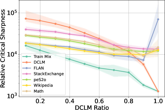
- Data-mix recommendations (e.g., the 0.6–0.7 DCLM “sweet spot”) were validated on OLMo-2 7B and specific datasets; expect shifts with other model sizes, curricula, token budgets, and evaluation targets.
Glossary
- AdamW: An Adam optimizer variant that decouples weight decay from the gradient-based update to improve regularization. "during GPT-style Transformer training on FineWebEdu with AdamW using a Warmup-Stable-Decay (WSD) schedule."
- Adaptive optimizers: Optimizers (e.g., Adam) that adjust learning rates per-parameter using estimates of gradient statistics. "including mini-batch settings and adaptive optimizers, albeit governed by different notions of sharpness"
- Catastrophic forgetting: The degradation of performance on previously learned data/tasks when fine-tuning on new data. "neural networks are prone to catastrophic forgetting, where the model performance degrades on the pretraining dataset and benchmarks as the model adapts to the new task"
- Cosine decay: A learning rate schedule that decreases the rate following a cosine curve. "followed by a cosine decay down to one-tenth of its peak value"
- Critical learning rate: The smallest learning rate at which taking a step along the current update direction increases the loss. "defined as , where is the critical learning rate\textemdash the smallest learning rate that causes the training loss to increase in the next training step."
- Critical sharpness: A scalable curvature measure defined as two divided by the critical learning rate, capturing curvature along the optimizer’s update direction. "We analyze critical sharpness (), a computationally efficient measure requiring fewer than $10$ forward passes given the update direction ."
- Directional sharpness: A curvature measure along a specific update direction, approximating critical sharpness under a local quadratic model. "Directional sharpness $\lambda_{\text{dir}$ serves as an analytically tractable approximation to the empirically measured critical sharpness."
- Double backpropagation: Computing second derivatives via backpropagating through a first backpropagation pass. "second-derivative implementations required for double backpropagation."
- Edge of Stability (EoS): A training regime in which sharpness hovers around a critical threshold and loss does not diverge despite large learning rates. "the subsequent oscillations around the critical threshold is termed the Edge of Stability (EoS)"
- Edge of Stability threshold: The sharpness/learning-rate boundary that marks the onset of instability. "The dashed line denotes the Edge of Stability threshold, given by ."
- Eigendirection: A direction in parameter space corresponding to an eigenvector of a matrix (here, typically the Hessian). "where the weights quantify the alignment of the gradient with Hessian eigendirections ."
- Flash Attention: A highly optimized attention kernel for Transformers that often lacks second-derivative support. "kernels like Flash Attention \citep{dao2022flashattention} typically lack second-derivative implementations required for double backpropagation."
- Flatness: The reciprocal of Hessian sharpness; lower curvature implying a “flatter” loss region. "Its reciprocal, flatness , is a complementary measure used to describe the curvature."
- Hessian sharpness: The largest eigenvalue of the loss Hessian, indicating the worst-case local curvature and stability limit. "The most commonly studied measure, Hessian sharpness () \textemdash the largest eigenvalue of the loss Hessian \textemdash determines local training stability and interacts with the learning rate throughout training."
- Hessian-vector product (HVP): The product of the Hessian with a vector, used for curvature and eigenvalue estimation without forming the full Hessian. "require repeated Hessian-vector products (HVPs)."
- Lanczos: An iterative algorithm for approximating eigenvalues/eigenvectors, often used to estimate extreme eigenvalues of large matrices. "iterative eigenvalue solvers (e.g., Power iteration, Lanczos)"
- Learning rate warmup: A schedule phase that gradually increases the learning rate at the start of training to improve stability. "For the more realistic setting of learning rate schedules involving warmup and decay, sharpness closely follows the learning rate schedule"
- Line search: A procedure to choose a learning rate by evaluating loss along a proposed update direction. "To estimate the critical learning rate , we perform an efficient line search along the update direction from training."
- Power iteration: An iterative method to estimate the dominant eigenvalue and eigenvector of a matrix. "iterative eigenvalue solvers (e.g., Power iteration, Lanczos)"
- Pre-conditioned Hessian: The Hessian transformed by an optimizer’s pre-conditioner, reflecting the effective curvature under that optimizer. "the training dynamics is governed by the pre-conditioned Hessian "
- Pre-conditioned sharpness: The largest eigenvalue of the pre-conditioned Hessian, relevant for adaptive optimizers like Adam. "The pre-conditioned sharpness exhibits progressive sharpening"
- Pre-conditioner: A matrix (from an optimizer like Adam) that rescales gradients/parameters, altering the effective curvature. "For adaptive optimizers with pre-conditioner (e.g., Adam)"
- Pre-training basin: A region in parameter space where the pre-training loss remains low; leaving it indicates forgetting base capabilities. "helping the model stay near the ``pre-trained basin'' during finetuning."
- Progressive sharpening: The phenomenon where sharpness steadily increases during training until reaching the EoS. "The continual increase in Hessian sharpness is referred to as progressive sharpening"
- Quadratic loss approximation: A second-order Taylor approximation of the loss around current parameters, used to analyze local stability. "Under the quadratic loss approximation, we show that critical sharpness can be written as a weighted sum of Hessian eigenvalues"
- Rehearsal: A continual learning strategy that mixes prior (pre-training) data during fine-tuning to prevent forgetting. "Among these, rehearsal \textemdash mixing samples from the pre-training data \textemdash has become the most widely adopted strategy"
- Relative critical sharpness: A measure of how far one can move along updates from one objective before increasing another objective’s loss. "We further introduce relative critical sharpness (), which quantifies the curvature of one loss landscape while optimizing another"
- Self-stabilization mechanism: Dynamics whereby training avoids divergence at high sharpness by oscillating near the stability edge. "Once this threshold is reached, the training stabilizes through a self-stabilization mechanism"
- Stability threshold: The boundary (in terms of sharpness and learning rate) that separates stable from unstable training regimes. "we first analyze the stability threshold for common optimizers with weight decay"
- Warmup-Stable-Decay (WSD) schedule: A learning rate schedule with an initial warmup phase, a constant (stable) phase, and a final decay. "with Warmup-Stable-Decay (WSD) schedule."
- Weight decay: A regularization technique that shrinks parameters during training, often decoupled in AdamW. "Modern large-scale models are typically trained using Adam with weight decay~\citep{adamwloshchilov2018}"
Collections
Sign up for free to add this paper to one or more collections.

