Geometric Entanglement Entropy on Projective Hilbert Space
Abstract: Entanglement for pure bipartite states is most commonly quantified in a state-by-state manner to each pure state of a bipartite system a scalar quantity, such as the von Neumann entropy of a reduced density matrix. This provides a precise local characterization of how entangled a given state is. At the same time, this local description naturally invites a set of complementary, more global questions about the structure of the space of pure states: How abundant are the states with a given amount of entanglement within the full state space? Do the manifolds of constant entanglement exhibit distinct geometric regimes? These questions shift the focus from assigning an entanglement value to a single state to understanding the global organization and geometry of entanglement across the entire manifold of pure states. In this work, we develop a geometric framework in which these questions become natural. We regard the projective Hilbert space of pure states, endowed with the Fubini-Study metric, as a Riemannian manifold and promote bipartite entanglement to a macroscopic functional on this manifold. Its level sets stratify the space of pure states into hypersurfaces of constant entanglement, and we define a geometric entanglement entropy as the log-volume of these hypersurfaces, weighted by the Fubini-Study gradient of entanglement. This quantity plays the role of a microcanonical entropy in entanglement space: it measures the degeneracy of a given entanglement value in the natural quantum geometry. The framework is illustrated first in the simplest case of a single spin-1/2 and then for bipartite entanglement of spin systems, including a two-qubit example where explicit calculations can be carried out, along with a sketch of the extension to spin chains.

Paper Prompts
Sign up for free to create and run prompts on this paper using GPT-5.
Top Community Prompts
Explain it Like I'm 14
Plain-English Summary of “Geometric Entanglement Entropy on Projective Hilbert Space”
What is this paper about?
The paper looks at quantum entanglement from a new angle. Usually, scientists assign a number to a single quantum state to say “how entangled” it is. Instead, this paper asks a bigger, global question: across the whole set of possible quantum states, how common are states with a given amount of entanglement? To answer that, the author builds a geometric picture of the entire “space of quantum states” and defines a new quantity, called geometric entanglement entropy, that measures how many states share the same entanglement.
What questions is the paper trying to answer?
The paper focuses on simple, global questions about entanglement:
- How many pure states have a specific amount of entanglement?
- Do the sets of states with equal entanglement have special geometric shapes or “phases”?
- How quickly does entanglement change when you slightly tweak a state?
How do they study it? (The main ideas and tools)
Think of the set of all pure quantum states as a landscape:
- The “projective Hilbert space” is the map of all possible pure states (ignoring an overall unimportant phase).
- The “Fubini–Study metric” is a built-in way to measure distance and area on that map, like measuring distances and areas on a globe.
Now, imagine drawing contour lines on this map:
- Pick a standard entanglement measure (for a bipartite system, it’s the von Neumann entropy of one part). This is just a function that gives each state a number (its entanglement).
- The set of all states that have the same entanglement is like a contour line (or, in higher dimensions, a “surface”) on the map.
The paper then borrows a classic idea from statistical physics:
- In thermodynamics, entropy is related to how many microstates have the same energy (the size of an “energy shell”).
- Here, replace “energy” with “entanglement,” and measure the size of each constant-entanglement surface using the Fubini–Study metric.
- The “geometric entanglement entropy” is the logarithm of this size. It tells you how abundant states with that entanglement are, in the natural geometry of quantum states.
To connect geometry and change:
- The paper also looks at “curvature” of those surfaces (how bent they are, like the shape of a hill).
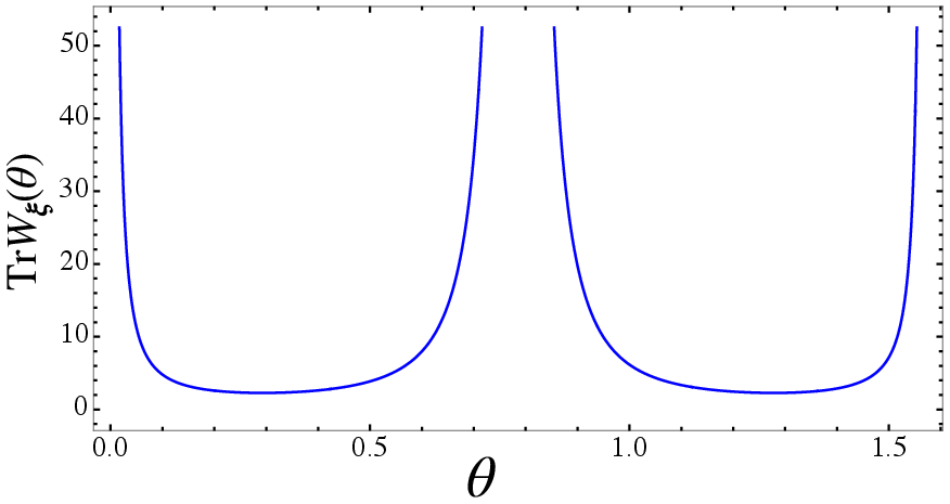
- A specific curvature quantity (mean curvature, captured by something called the Weingarten map) tells you how the size of the constant-entanglement surface changes when you move to nearby surfaces with slightly different entanglement.
What did they actually do? (Methods and examples)
To make the framework concrete, the paper:
- Explains the Fubini–Study geometry in simple cases.
- Shows a warm-up with a single qubit: the state space is the Bloch sphere (a sphere where each point is a pure state). This sets the geometric stage.
- Studies two qubits: any pure state can be summarized by one angle (the Schmidt angle), which controls the entanglement. The paper calculates:
- The Fubini–Study metric on this two-parameter family of states.
- The “size” (volume) of the set of states with the same entanglement.
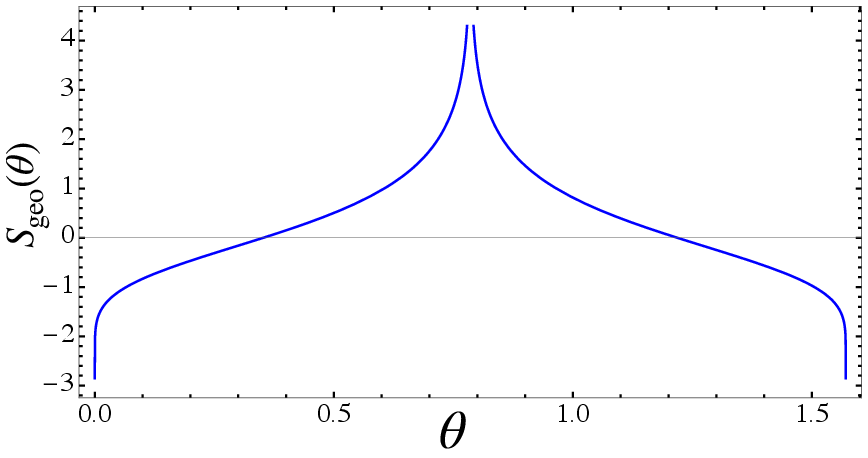
- The geometric entanglement entropy S_geo(e) = log(size).
- How the slope of S_geo with respect to entanglement equals an average curvature of the constant-entanglement surfaces. In everyday terms: how quickly the “abundance” changes with entanglement is controlled by how curved those surfaces are.
Finally, the paper sketches how this extends to many spins (spin chains), where the state space is huge and very rich.
What are the main findings and why do they matter?
- A new definition: geometric entanglement entropy S_geo(e) that counts how many pure states (in the natural quantum geometry) share the same entanglement e. This is different from the usual entanglement entropy E(state), which rates a single state.
- A microcanonical-style formula: just like energy shells in thermodynamics, the “entanglement shells” have a size (volume), and S_geo is the log of that size.
- A curvature link: the rate at which S_geo grows with entanglement equals a geometric curvature average of those constant-entanglement surfaces. Intuitively, how fast the “abundance” changes is controlled by how the surfaces bend.
- Two-qubit takeaway: in the natural geometry of state space, weakly entangled (almost product) states are extremely rare (tiny volume), while nearly maximally entangled states are very common (large volume). This puts a precise geometric meaning behind the familiar idea that “random” pure states are typically highly entangled.
Why is this important? (Implications and impact)
- A global view of entanglement: Instead of rating states one by one, we get a full map of how entanglement is distributed across all pure states.
- A unifying geometric language: This framework connects quantum information (entanglement) with differential geometry (metrics, volumes, curvature), opening new ways to analyze “entanglement landscapes.”
- Insight for many-body physics: It offers a clean, model-independent way to talk about entanglement “phases” and typicality, which could help understand complex systems (like spin chains) and phenomena such as entanglement transitions.
- Practical perspective: Since highly entangled states are geometrically abundant, this supports why random circuits tend to generate lots of entanglement and why special structures (like area-law states) are rare and thus valuable for efficient simulations and quantum technologies.
In short: the paper turns entanglement into a geometric, global concept. It shows how to measure “how many states” have a given entanglement, ties that count to curvature, and demonstrates that high entanglement is typical in the natural geometry of quantum state space.
Knowledge Gaps
Below is a concise list of concrete knowledge gaps, limitations, and open questions that remain unresolved in the paper. These items are intended to guide future research efforts.
- Rigorous treatment of singular values of the entanglement functional E on projective Hilbert space:
- Formal conditions under which the coarea formula applies to E, including handling of critical points where ∥∇E∥ vanishes (e.g., near product states and maximally entangled states).
- Regularization or geometric stratification of level sets Σe at non-regular values (e.g., cusp-like behavior at maximal entanglement).
- Dependence on the choice of metric and measure:
- Sensitivity of S_geo(e) and ω(e) to replacing the Fubini–Study measure with other unitarily invariant measures (e.g., Bures, Hilbert–Schmidt).
- Invariance of qualitative conclusions (e.g., abundance of high entanglement) under metric scaling and normalization choices.
- Local-unitary orbit quotienting:
- Explicit construction of S_geo(e) on the quotient manifold P(H)/(SU(d_A)×SU(d_B)) to factor out local-unitary redundancies.
- Comparison between counting on full projective space versus the orbit space of Schmidt spectra (to avoid overcounting physically equivalent states).
- Full CPd−1 computation in the two-qubit case:
- Calculation of ω(e) over the entire CP3 (not just the reduced Schmidt family) to verify the cusp and divergence features suggested by the reduced model.
- Analytical or numerical benchmarking against known distributions of Schmidt coefficients for random two-qubit states.
- Asymptotics and large-N behavior for many-body systems:
- Derivation of S_geo(e) for large N and various bipartition ratios (d_A/d_B), using random matrix theory and large-deviation methods (e.g., Wishart spectra).
- Precise characterization of how area-law, logarithmic, and volume-law entanglement regimes are represented in S_geo(e), including scaling forms and concentration phenomena.
- Curvature-based “entanglement phases”:
- Clear, testable definitions of entanglement “phases” in terms of intrinsic/extrinsic curvature invariants of Σe (e.g., mean/scalar curvature thresholds).
- Identification of geometric transition points in S_geo(e) and their relation to known entanglement phase transitions (e.g., monitored circuits, random dynamics).
- General proof of the entropy–curvature relation:
- A rigorous, global proof on projective Hilbert space that ∂e S_geo(e) equals the microcanonical average of the Weingarten trace for arbitrary E, beyond the worked two-qubit example.
- Computational methodology:
- Practical algorithms (Monte Carlo/coarea-based samplers) to estimate ω(e) and curvature invariants on Σe in high-dimensional manifolds.
- Numerical stability near regions where ∥∇E∥ is small and the Jacobian factors in the coarea formula blow up.
- Extension to mixed states and alternative entanglement measures:
- Generalization of the framework to mixed states (e.g., density matrices with Bures metric) and measures like negativity, entanglement of formation, or Rényi entropies.
- Comparison of S_geo(e) across different entanglement monotones and their operational interpretations.
- Multipartite entanglement:
- Extension from bipartite cuts to genuinely multipartite settings (e.g., entanglement polytopes, SLOCC classes) and corresponding geometric entropies.
- How S_geo(e) interacts with majorization and entanglement monotone hierarchies in multipartite systems.
- Physical interpretability and operational relevance:
- Connection between S_geo(e) and resource-theoretic tasks (distillation, conversion rates), and whether S_geo(e) predicts operational “typicality” or cost.
- Relation between entanglement growth under unitary or monitored dynamics and geometric flux across Σe; formulation of dynamical continuity equations in “entanglement space.”
- Robustness to subsystem choice:
- Systematic study of how S_geo(e) depends on the bipartition (size, geometry of A), including universality or non-universality across partitions.
- Infinite-dimensional and QFT extensions:
- Adaptation to continuous-variable systems and QFT (where entanglement is UV-divergent), including renormalization of S_geo(e) and metric issues on infinite-dimensional projective spaces.
- Normalization and scaling of S_geo:
- Definition of dimensionless or per-degree-of-freedom versions of S_geo(e) for meaningful comparison across system sizes.
- Clarification of additive constants and scaling dependence, especially when comparing different metrics or dimensions.
- Relationship to known typicality results:
- Explicit linkage of S_geo(e) to Page’s theorem and known entanglement distributions, providing closed-form or asymptotic expressions where possible.
- Geometry of Σe beyond mean curvature:
- Computation and interpretation of higher curvature invariants (e.g., Gaussian/scalar curvature, principal curvatures) on Σe and their impact on ω(e).
- Intersections with physical constraints:
- Joint geometric entropy for intersections of Σe with other macroscopic constraints (e.g., fixed energy shells), and how combined constraints reshape entanglement typicality.
Collections
Sign up for free to add this paper to one or more collections.

