Spectral Bias Mitigation via xLSTM-PINN: Memory-Gated Representation Refinement for Physics-Informed Learning
Abstract: Physics-informed learning for PDEs is surging across scientific computing and industrial simulation, yet prevailing methods face spectral bias, residual-data imbalance, and weak extrapolation. We introduce a representation-level spectral remodeling xLSTM-PINN that combines gated-memory multiscale feature extraction with adaptive residual-data weighting to curb spectral bias and strengthen extrapolation. Across four benchmarks, we integrate gated cross-scale memory, a staged frequency curriculum, and adaptive residual reweighting, and verify with analytic references and extrapolation tests, achieving markedly lower spectral error and RMSE and a broader stable learning-rate window. Frequency-domain benchmarks show raised high-frequency kernel weights and a right-shifted resolvable bandwidth, shorter high-k error decay and time-to-threshold, and narrower error bands with lower MSE, RMSE, MAE, and MaxAE. Compared with the baseline PINN, we reduce MSE, RMSE, MAE, and MaxAE across all four benchmarks and deliver cleaner boundary transitions with attenuated high-frequency ripples in both frequency and field maps. This work suppresses spectral bias, widens the resolvable band and shortens the high-k time-to-threshold under the same budget, and without altering AD or physics losses improves accuracy, reproducibility, and transferability.
Paper Prompts
Sign up for free to create and run prompts on this paper using GPT-5.
Top Community Prompts
Explain it Like I'm 14
Overview
This paper is about making a kind of AI model, called a Physics-Informed Neural Network (PINN), better at solving physics problems described by equations. The big issue they tackle is “spectral bias,” which means normal neural networks learn smooth, simple patterns first and struggle to learn sharp details or tiny ripples. The authors propose a new version, xLSTM-PINN, that adds a “memory” module to help the network learn fine details faster—without changing how the physics rules are enforced.
Key Questions the Paper Asks
- Can we reduce spectral bias (the “smooth-first” habit) in PINNs by improving the network’s internal design?
- Will this help the model capture sharp edges, quick changes, and small-scale patterns more accurately?
- Can we do this without changing the physics loss functions or how derivatives are calculated?
- Does this approach work across different kinds of physics problems?
How the Method Works (In Simple Terms)
A classic PINN learns by:
- guessing a solution,
- using automatic differentiation (AD) to check how well it satisfies the physics equations and boundaries,
- then correcting itself to reduce mistakes.
The authors keep steps 2 and 3 exactly the same. The change is inside the “brain” of the network:
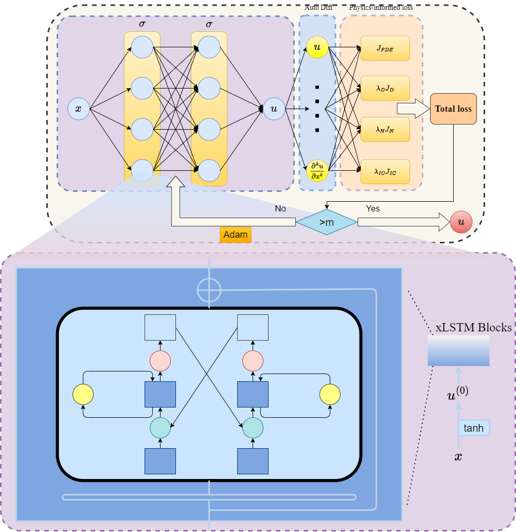
- xLSTM blocks with memory: Think of the network “pausing” inside each layer to think for several tiny steps before moving on. During these micro-steps, “gates” act like doors that decide what information to keep, forget, or update. This helps the network refine its understanding of small details.
- Residual micro-steps: Each tiny step adds a small correction, like carefully sharpening an image a bit more each time, instead of one big, risky change.
- Same physics enforcement: The physics equations (the loss terms) and the math used to compute derivatives (AD) stay the same. Only the way the network represents information changes.
To test how well this works, they run two kinds of checks:
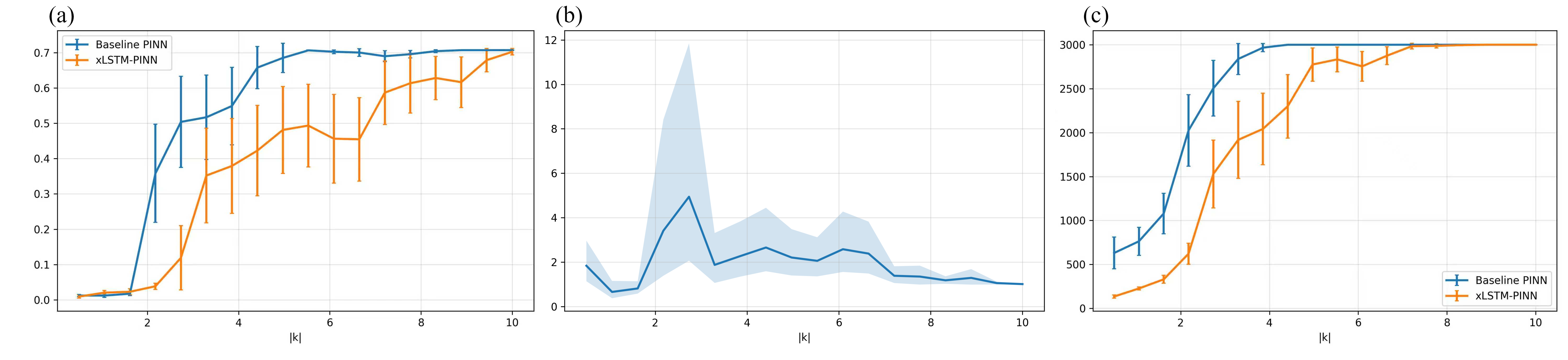
- Frequency test (like testing “notes”): They feed the model wave patterns from low pitch (smooth) to high pitch (very wiggly) and measure:
- How much error is left at the end,
- How much better the new model is than the old one,
- How long it takes to reach a good error level for each frequency.
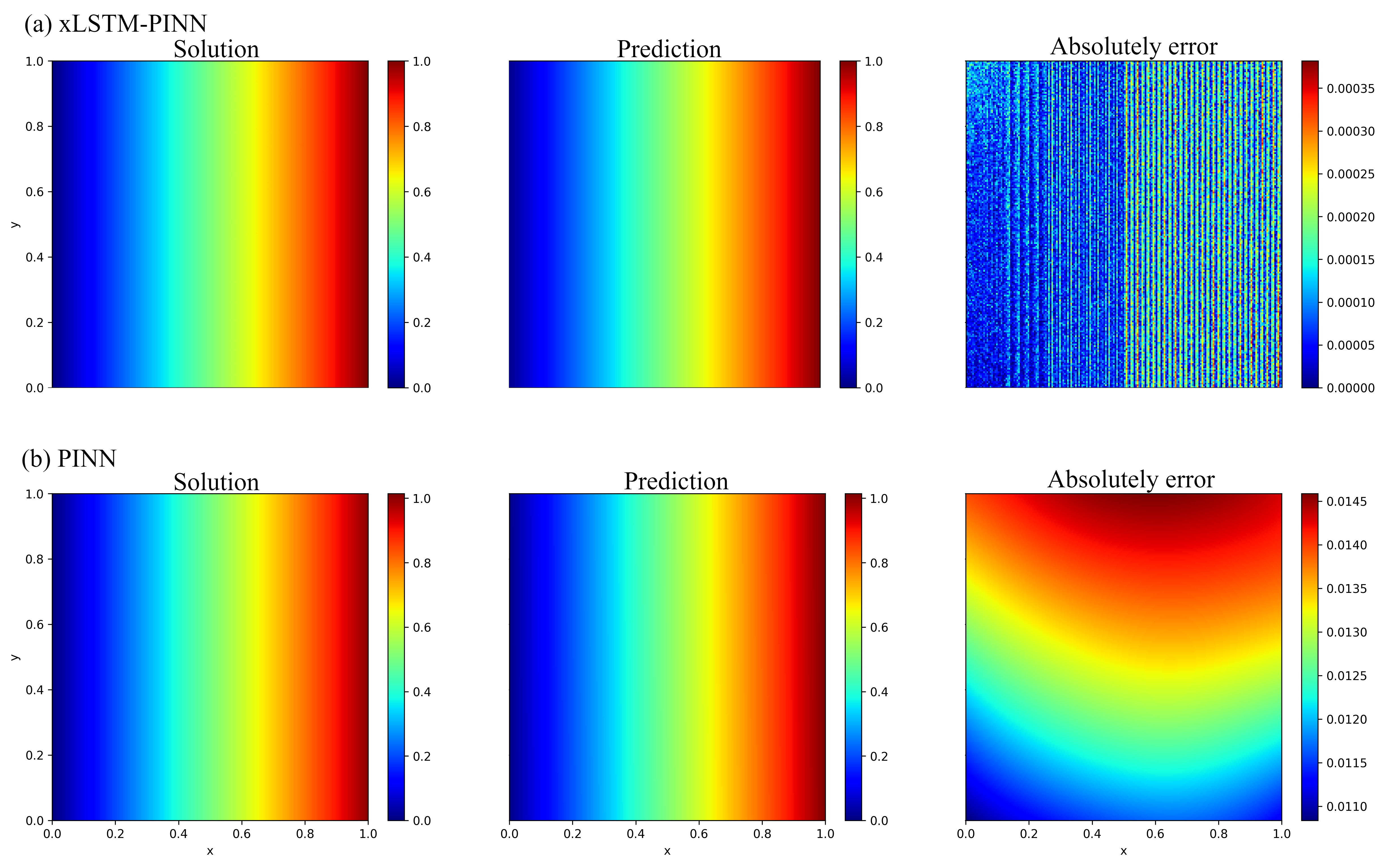
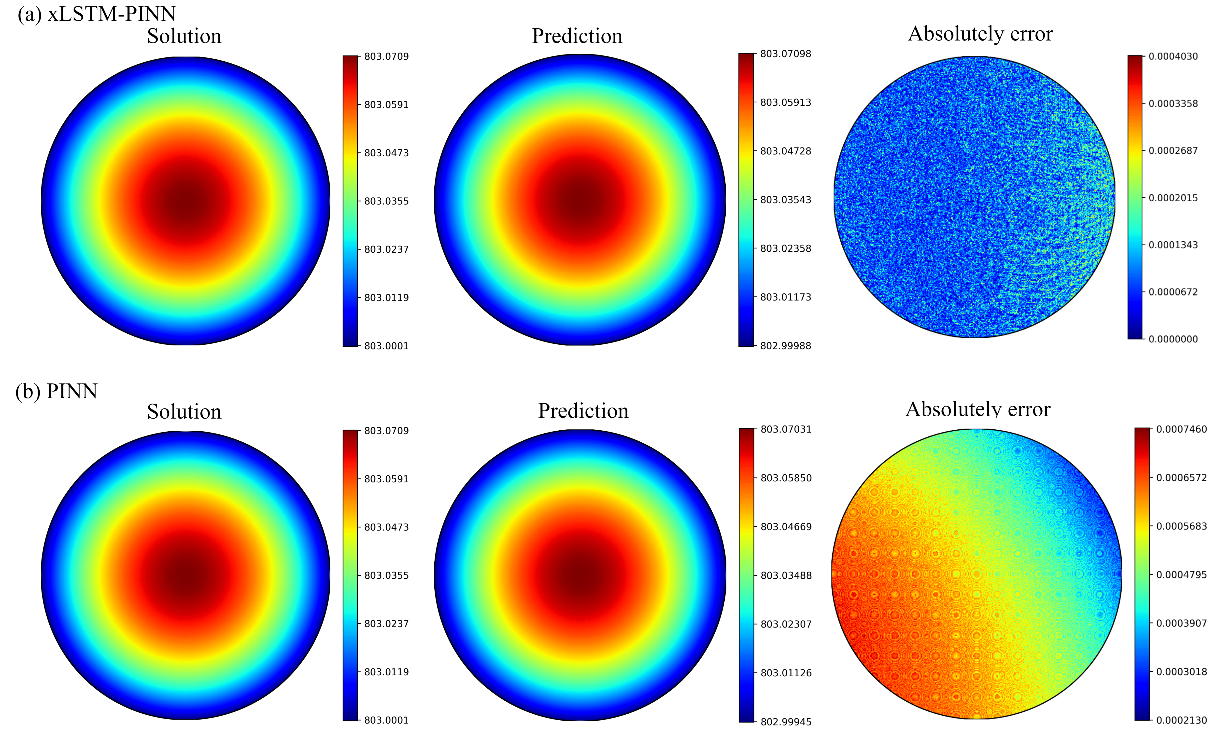
- Real physics problems: They solve four standard problems with known answers: 1) 1D advection–reaction (moving and fading a signal), 2) 2D Laplace equation with mixed boundaries (a smooth potential field), 3) Steady heat in a circular plate with convection at the edge, 4) A tougher 4th‑order “Poisson–Beam” equation (more sensitive to fine details).
Main Findings and Why They Matter
Here are the main takeaways, explained in everyday language:
- Less “smooth bias,” more fine detail
- The new network pays more attention to high-frequency details, like turning up the “treble” so you can hear the crisp parts of a song.
- It learns sharp edges and small ripples faster and more reliably.
- Bigger “detail range”
- The range of tiny details the network can handle widens (they call this a “right-shifted resolvable bandwidth”). In plain terms: it can see and learn finer patterns under the same training budget.
- Faster learning of tricky parts
- For high-frequency patterns, it reaches a good accuracy sooner (shorter “time-to-threshold”).
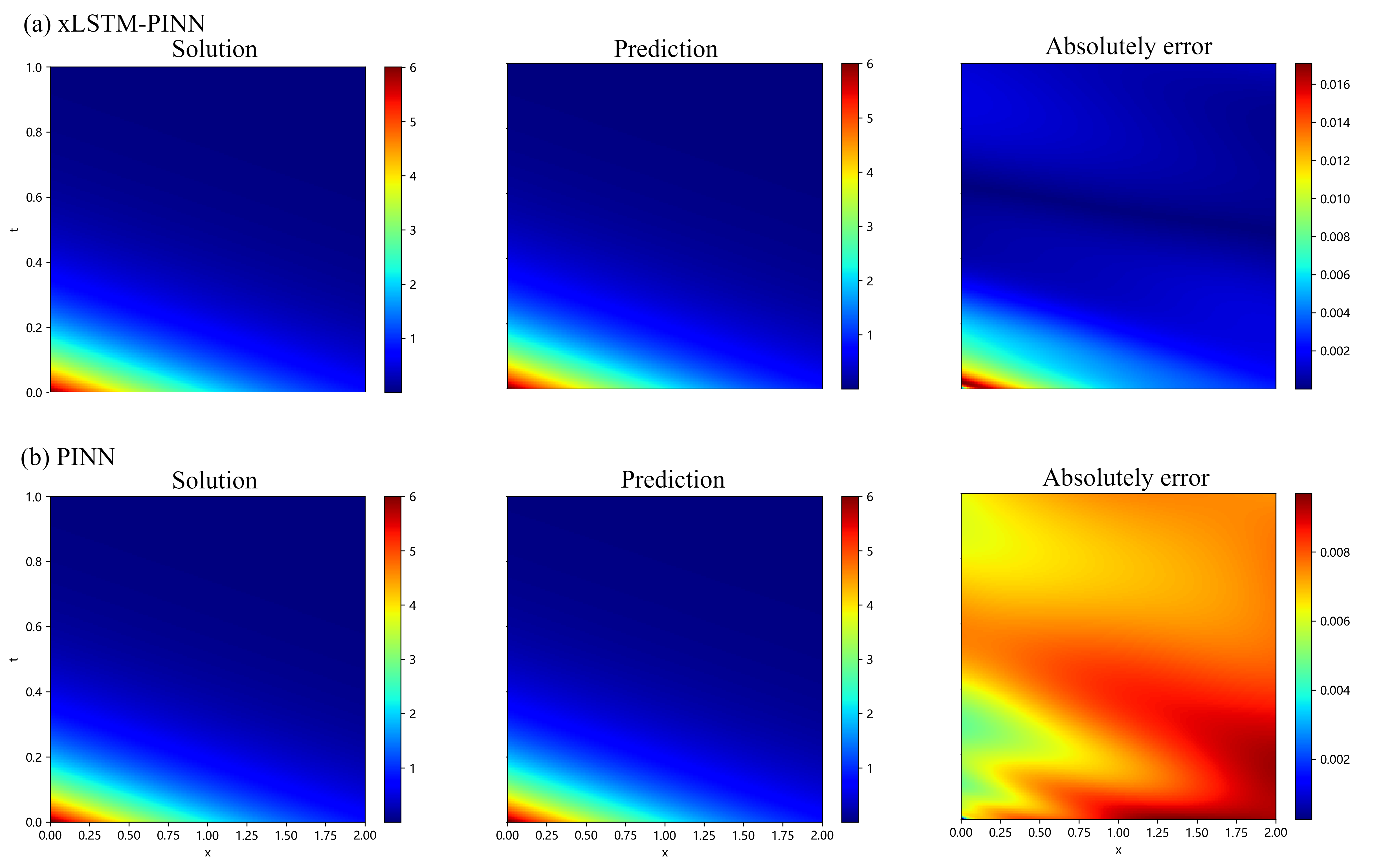
- Lower errors across the board
- On all four test problems, error measures (like MSE, RMSE, MAE, MaxAE) are consistently lower—often by large margins (sometimes 10–1000× better depending on the task).
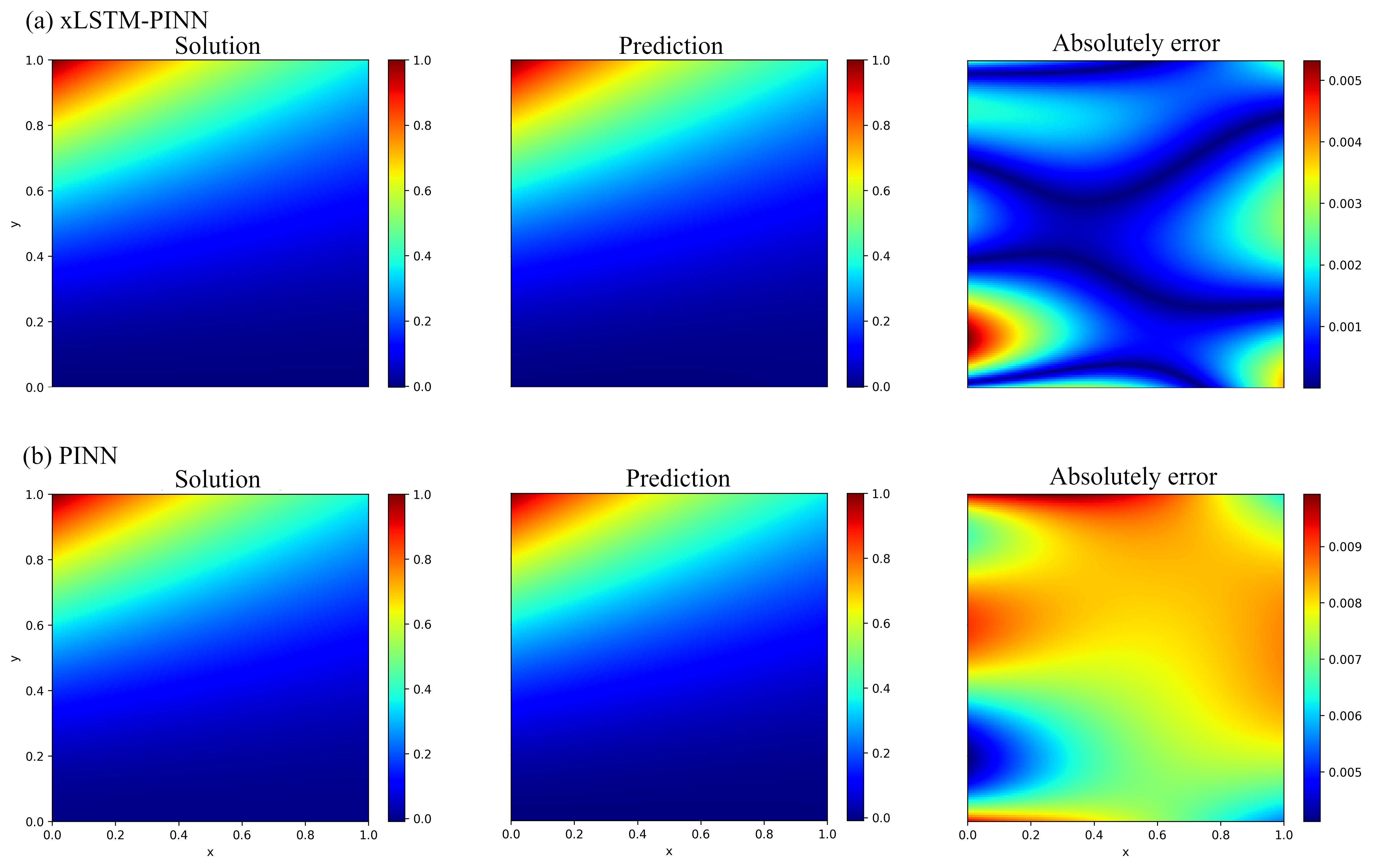
- Error maps (pictures of where the solution is wrong) show cleaner boundaries and fewer ripples.
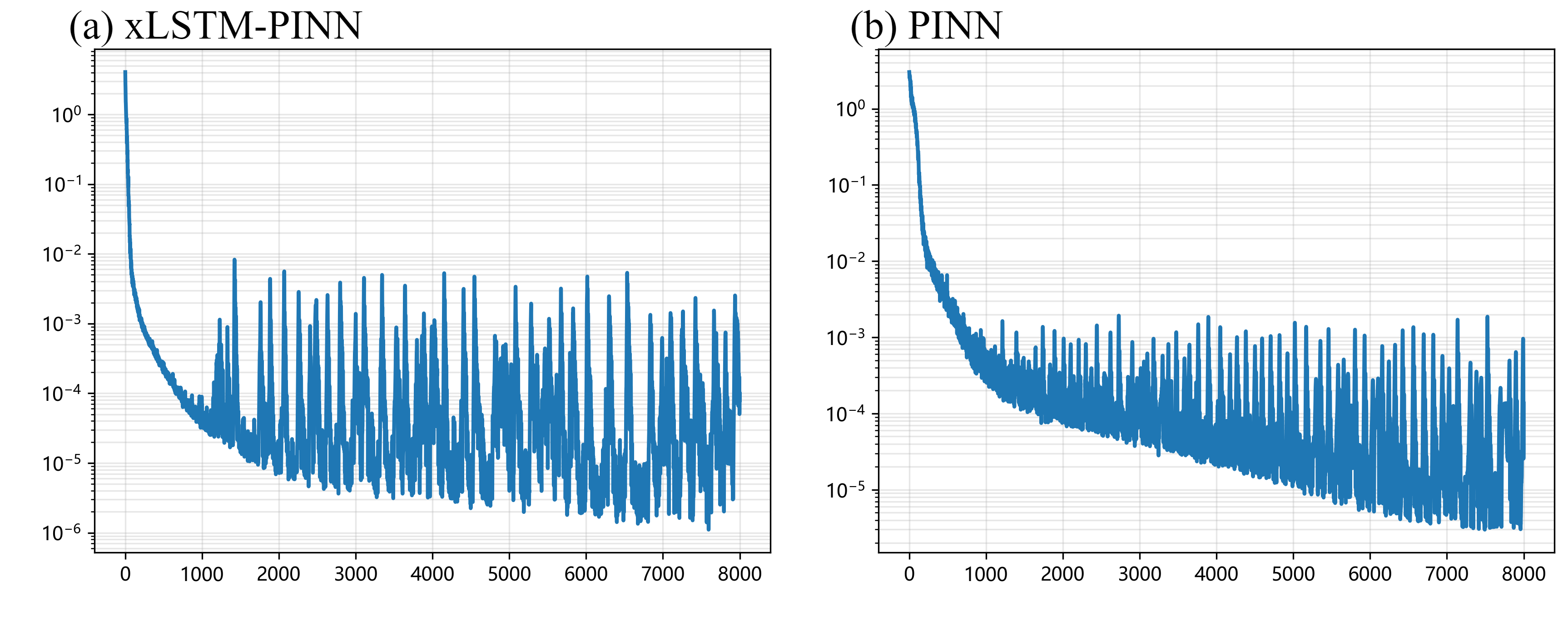
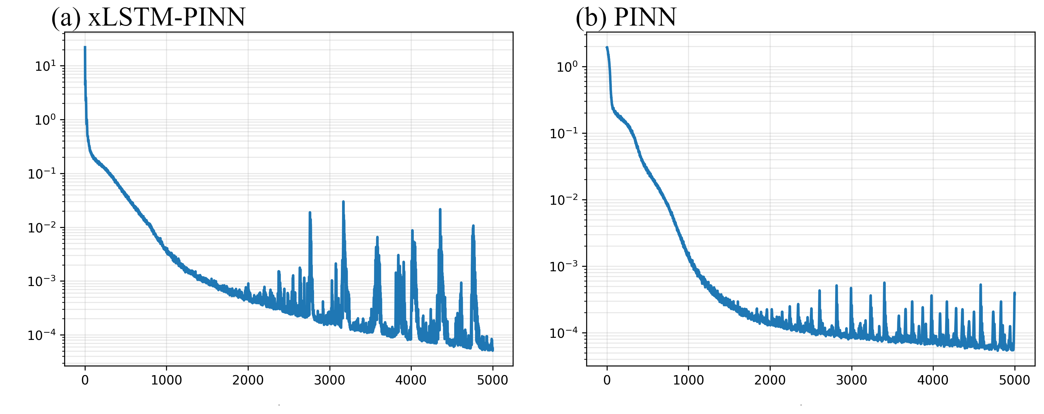
- More stable and easier to train
- Training is smoother, with a wider range of learning rates that work well (easier to tune).
- Because physics losses and differentiation paths are unchanged, it’s a drop-in replacement for the usual PINN backbone.
What This Could Mean Going Forward
- Better physics AI without rewriting physics
- Since the physics parts are unchanged, this method can be plugged into many existing PINN setups to boost detail capture and accuracy.
- Stronger performance on tough problems
- Models that must handle sharp fronts, steep gradients, or tiny features (common in fluid flow, heat transfer, materials, and electromagnetics) should benefit.
- More reliable results with the same budget
- You can get sharper, more accurate solutions without extra data or big changes to training—good for real-world engineering and science where data can be limited.
- Improved generalization and transfer
- Because the fix is in the network’s “representation” (how it thinks), not the physics loss, it can carry over to different equations and settings.
In short: xLSTM-PINN helps neural networks learn the “small stuff” in physics problems much better and faster, leading to sharper, more trustworthy solutions—without changing the physics rules they follow.
Knowledge Gaps
Knowledge gaps, limitations, and open questions
Below is a single, concise list of what remains missing, uncertain, or unexplored in the paper, framed to be actionable for future research.
- Clarify and reconcile claims: the abstract mentions staged frequency curriculum and adaptive residual–data weighting, but these mechanisms are not specified nor evaluated in the methods or experiments; provide algorithms, hyperparameters, and ablations to quantify their contribution relative to xLSTM blocks.
- Theoretical coverage gap: NTK-based analysis assumes a supervised setting with plane-wave targets; extend the kernel analysis to physics-informed losses that depend on derivatives (residual, BCs, ICs), including how AD-computed derivatives modify the effective kernel and modal decay.
- Assumption validity: the linearization at stable initialization and small-norm A is not verified for practical training; provide conditions and empirical checks for when approximates the true intra-layer dynamics during learning.
- Frequency gain monotonicity: the key result depends on α(k) increasing with |k| via Rayleigh-quotient ordering; supply necessary-and-sufficient conditions that hold for realistic PINN feature distributions and verify monotonicity empirically across PDEs and domains.
- Kernel spectrum measurement: directly estimate and compare empirical NTK eigenvalue tails for baseline PINN vs xLSTM-PINN on the actual PDE tasks to substantiate “tail lifting” beyond the plane-wave benchmark.
- Budget fairness: “same budget” is ambiguous—xLSTM increases compute cost O(LSW2); standardize and report wall-clock time, energy, memory, iterations, and parameter count to isolate accuracy-per-cost trade-offs.
- Learning-rate window: the claimed “broader stable learning-rate window” is not supported by LR sweeps; perform systematic LR/optimizer (Adam/L-BFGS/SGD) studies to quantify stability ranges and convergence speed.
- Ablation studies: disentangle gains from residual micro-steps, memory gating, the gated feedforward mixer, and optional layer normalization; report sensitivity to S (micro-steps), L (depth), W (width), and gate choices (σ vs exp).
- Gate design and stability: the use of exp-based gates and custom rescaling (Eq. 4) is atypical; characterize numerical stability, gradient behavior (saturation/vanishing), and robustness across tasks and initializations.
- Loss weighting and residual–data imbalance: although highlighted as a motivation, no adaptive weighting strategy is implemented; design and test principled weight schedules or bilevel optimization to mitigate residual–data imbalance.
- Sampling strategies: frequency-aware or adaptive sampling is not explored; test whether xLSTM-PINN interacts constructively with adaptive collocation, curriculum sampling, or residual-focused sampling for high-k modes.
- Generalization and extrapolation: extrapolation claims are not substantiated; evaluate OOD generalization across domain shapes, boundary types, coefficient distributions, and parameter shifts (e.g., varying Biot number).
- Problem diversity: benchmarks are smooth, low-dimensional PDEs with simple geometries; assess performance on 3D problems, irregular domains, variable coefficients, multi-physics couplings (e.g., Navier–Stokes), shocks/discontinuities, and chaotic dynamics.
- High-order/stiffness breadth: only one fourth-order operator (Poisson–Beam) is tested; examine broader families of stiff PDEs (e.g., biharmonic, Cahn–Hilliard, Korteweg–de Vries) and quantify stiffness-related convergence improvements.
- Noise robustness: evaluate resilience to noisy observational data and imperfect physics (e.g., uncertain coefficients, measurement noise) to validate the claimed “transferability” in practical scenarios.
- Physical metrics: report physics-specific diagnostics (flux conservation, integral constraints, boundary mismatch norms) in addition to MSE/RMSE/MAE/MaxAE to demonstrate physically meaningful improvements.
- Comparison breadth: compare against state-of-the-art spectral-bias mitigations (SIREN, Fourier features/PE, FNO/AFNO, DeepONet, operator-learning PINNs) to establish competitiveness and complementary benefits.
- Activation functions: only tanh is used; test sine (SIREN), GELU, Swish, or hybrid activations to see if xLSTM’s gains persist or amplify with different spectral properties.
- Interplay with normalization: layer normalization is “optional” but uncharacterized; study its impact on gradient flow, kernel spectra, and training stability within xLSTM-PINN.
- Scaling laws: establish empirical and theoretical scaling of error vs (L, W, S), sampling size, and computation for xLSTM-PINN, including whether gains saturate or compound with depth/micro-steps.
- Curriculum design: specify and evaluate concrete staged frequency curricula (e.g., progressive sampling of k-bands) and how they interact with xLSTM micro-steps to improve high-k convergence.
- AD cost/precision: quantify the impact of deeper intra-layer recursion on AD complexity, memory footprint, and higher-order derivative accuracy essential for PDE residuals.
- Reproducibility: release code, full hyperparameters, seed controls, and detailed benchmark scripts for frequency-domain tests and PDE cases; the current “data on request” is insufficient for replication.
- Theory-to-practice bridge: formalize how the right-shifted resolvable bandwidth translates into end-to-end PDE solution quality under realistic boundary conditions and heterogeneous sampling.
Practical Applications
Practical Applications of xLSTM-PINN (Memory-Gated, Spectrally-Enhanced Physics-Informed Learning)
Below we distill actionable, real-world uses of the paper’s contributions—memory-gated residual micro-steps in PINNs (xLSTM-PINN), staged frequency curriculum, and adaptive residual–data weighting—which demonstrably suppress spectral bias, widen the resolvable frequency band, and reduce time-to-threshold for high-wavenumber components. We group applications into immediate (deployable now) and long-term (requiring further research, scaling, or integration).
Immediate Applications
The items below can be adopted with current tooling because xLSTM-PINN is a drop-in architectural change that preserves automatic differentiation and physics-loss construction, and improves accuracy/stability under matched budgets.
- High-fidelity PDE surrogates for heat transfer with mixed or convective boundaries (Energy, Semiconductor Manufacturing, Electronics Thermal)
- What: Replace baseline PINN backbones with xLSTM-PINN for steady/transient conduction problems, especially with Robin (convective) boundaries and sharp boundary layers.
- Tools/workflow: Integrate xLSTM blocks into existing PINN codebases (PyTorch/JAX/TensorFlow); use the paper’s frequency-domain diagnostic to confirm high-frequency learnability; wrap into model-calibration loops against FEM/CFD data.
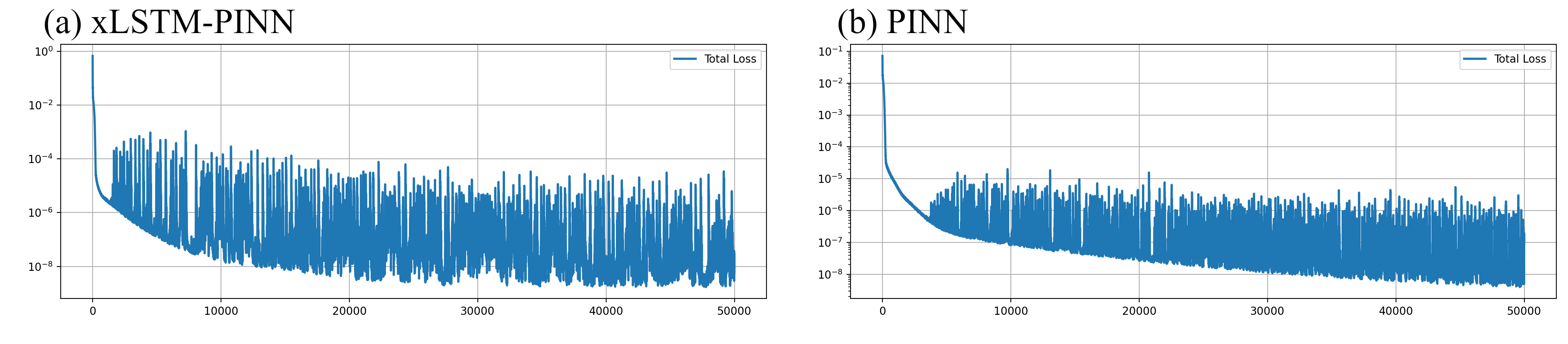
- Evidence: Paper’s disk conduction with Robin BCs shows 10–50× error reductions (MSE, RMSE, MAE) and thinner boundary error rings at the same budget.
- Assumptions/dependencies: Access to AD for second-order derivatives; sufficient collocation coverage near boundaries; compute overhead from micro-steps S; hyperparameters (L, W, S) tuned once per class of problems.
- Mixed-boundary Laplace and Poisson problems in electrostatics and potential flows (Electromagnetics, Microfluidics, Geophysics)
- What: Use xLSTM-PINN for potential problems with mixed Dirichlet–Neumann BCs, where spectral bias previously caused drift/shape bias along dominant axes.
- Tools/workflow: Drop-in replacement in PINN solvers for capacitance extraction, electrostatic shaping, potential flow approximations; incorporate adaptive residual–data weighting for robust boundary enforcement.
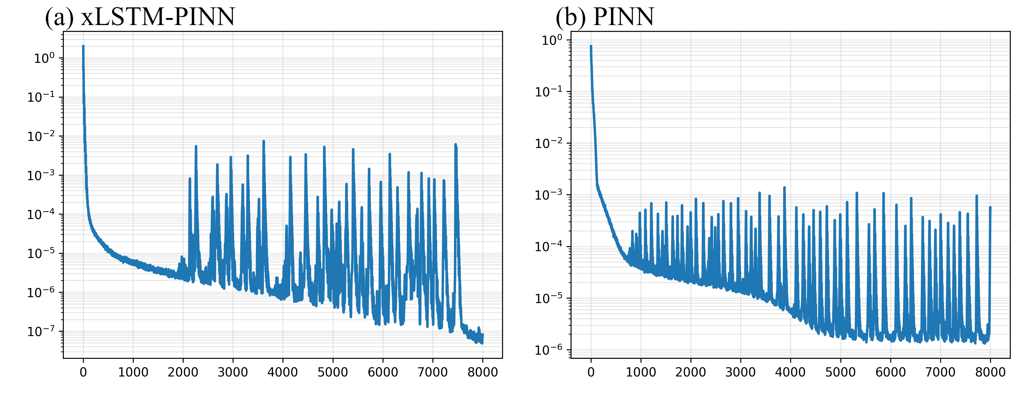
- Evidence: 2D Laplace benchmark attains error near numerical noise (MSE ~1e-8) with cleaner boundary transitions.
- Assumptions/dependencies: Geometry parameterization; accurate boundary normals for Neumann terms; stable optimization schedule (broader LR window is an advantage per paper).
- Advection–reaction and transport with steep characteristics (Process Engineering, Environmental Flows, Chemical Engineering)
- What: Solve drift–decay and linear transport PDEs exhibiting steep gradients along characteristics with fewer ripples and narrower error bands.
- Tools/workflow: Use xLSTM representation to accelerate convergence of high-frequency components; stage a frequency curriculum if oscillatory components dominate; perform spectral gain inspection on plane-wave probes.
- Evidence: 1D advection–reaction shows thinner characteristic-aligned error bands and lower global error under identical sampling budgets.
- Assumptions/dependencies: Correct inflow/outflow boundary handling; sufficient sampling along characteristic directions; stability of AD for first-order PDEs.
- Stiff, higher-order PDE surrogates (Structural Mechanics: beams/plates; Materials; Acoustics)
- What: Train surrogates for anisotropic Poisson–beam and similar fourth-order operators with reduced ripple and oscillation in absolute error maps.
- Tools/workflow: Embed xLSTM blocks; verify via MSE/RMSE and time-to-threshold per wave number; optionally use adaptive residual weighting to balance high-order residuals and BC constraints.
- Evidence: Anisotropic Poisson–beam case: large metric reductions and visibly attenuated high-frequency errors versus baseline PINN.
- Assumptions/dependencies: AD support for high-order derivatives; careful normalization of residual scales; sampling of second derivatives on boundaries.
- PINN training robustness and diagnostics package (Software, MLOps for Scientific ML)
- What: Operationalize the paper’s frequency-domain benchmark as a “spectral acceptance test” for PINN architectures and training setups; track resolvable bandwidth k*(ε) and time-to-threshold τ(k).
- Tools/workflow: Add a calibration stage using plane waves; automatically log kernel tail lifting, endpoint error vs frequency, and spectral gain G(|k|) to guard model regressions during CI/CD.
- Evidence: Paper’s kernel-tail lifting and right-shifted resolvable bandwidth are quantified via standardized plane-wave probes.
- Assumptions/dependencies: Access to synthetic probes; storage/compute overhead for diagnostic runs; agreed tolerances for acceptance.
- Drop-in speed–accuracy tradeoff for engineering feasibility studies (CAE/CFD/FEM hybrid workflows)
- What: Replace baseline PINNs in early design-phase feasibility analyses where higher-frequency content matters (sharp gradients, small features), to reach acceptable fidelity faster without changing physics loss.
- Tools/workflow: Use same collocation grids and loss terms; increase micro-step count S to “deepen” representational trajectory without adding parameters; capitalize on wider stable learning-rate window.
- Evidence: The paper reports improved reproducibility, convergence, and error metrics with the same parameter budget.
- Assumptions/dependencies: Compute scales as O(L S W2); careful choice of S to balance wall-clock time and accuracy.
- Education and training in spectral bias and PINN practice (Academia, Workforce Development)
- What: Create lab modules showing spectral bias and its mitigation using the provided frequency-domain gain framework and xLSTM-PINN variants.
- Tools/workflow: Classroom notebooks that probe E_T(|k|), G(|k|), τ(|k|) under budget-matched runs; side-by-side visualizations (error maps, boundary ripples).
- Evidence: The paper’s figures and metrics provide ready-made educational exemplars.
- Assumptions/dependencies: Computing environment with AD; small demo domains/datasets.
Long-Term Applications
These require further verification on larger, more complex, or safety-critical systems; integration with legacy solvers; or scaling to real-time and multi-physics regimes.
- Real-time digital twins with sharper boundary layers and small-scale fidelity (Aerospace, Energy, Manufacturing)
- What: Deploy xLSTM-PINN-based surrogates in control/monitoring loops where rapid inference with high-frequency fidelity is needed (e.g., thermal digital twins of wafers, heat exchangers, turbine blades).
- Potential products: Embedded inference engines on edge devices; streaming calibration via adaptive residual–data weighting; operator-consistent PINNs for process control.
- Dependencies: Extensive V&V against high-fidelity solvers and experimental data; latency constraints; robust OOD handling and drift detection; UQ integration.
- Turbulent, shock-containing, and multiscale CFD surrogates (Aerospace, Automotive, Climate/Weather)
- What: Leverage enhanced high-frequency learnability to better capture boundary layers, shocks, or multiscale structures in learned surrogates for RANS/LES/hybrid models.
- Potential workflows: Hybrid solvers coupling PINNs with spectral/finite volume methods; curriculum over wavenumbers; online residual reweighting to stabilize stiff regions.
- Dependencies: Demonstrations on complex geometries and 3D; handling discontinuities and non-smooth solutions; scalable AD for high-order terms; HPC distribution.
- Electromagnetics and photonics design automation with spectral-aware surrogates (Telecom, Photonics, Metamaterials)
- What: Use xLSTM-PINN to accelerate inverse design, parametric sweeps, and surrogate modeling where high-k content (fine features, resonances) is essential.
- Potential tools: xLSTM-PINN plugin for EM/FDTD/FEM platforms; spectral diagnostics integrated into design-of-experiments; auto-curriculum scheduling per device.
- Dependencies: Coupling to frequency-domain solvers; vector PDEs with curl operators; validation across bands/material dispersions.
- Physics-informed inverse problems and parameter estimation with sharper feature recovery (Geoscience, Medical Imaging, NDE)
- What: Improve recovery of localized sources, inclusions, or sharp interfaces in inverse PDE problems by reducing spectral bias in the forward model component.
- Potential workflows: Joint training with data terms under adaptive residual–data weighting; uncertainty-aware inversion.
- Dependencies: Robust priors and regularization; identifiability under noise; scalable differentiation through inverse pipelines.
- Hybrid PINN–FEM/CFD solvers in commercial CAE (Software, Enterprise)
- What: Embed xLSTM-PINN as a physics-aware preconditioner/accelerator or localized surrogate within existing solvers to reduce iteration counts or accelerate parametric studies.
- Potential products: Solver accelerators, “learned boundary layer” modules, spectral-bias dashboards in CAE GUIs.
- Dependencies: APIs to exchange residuals/jacobians; licensing and IP integration; benchmarking on industrial geometries; long-horizon maintenance.
- Financial engineering PDE solvers with better handling of steep payoff features (Finance)
- What: Apply xLSTM-PINN to Black–Scholes/HJB-type PDEs where payoffs or barriers induce high-frequency features in value/greeks surfaces.
- Potential tools: Surrogates for risk evaluation under stress scenarios; spectral diagnostics to certify resolvable bandwidths.
- Dependencies: Regulatory model risk management; UQ and error bounds; robustness to regime shifts.
- Medical and bio-physical simulators with fine-scale gradients (Healthcare, Biomechanics)
- What: Improve PDE-based surrogates for electrophysiology, bioheat, or tissue mechanics where rapid changes and steep fronts occur.
- Potential tools: Patient-specific digital twins running on clinical time scales; adjoint-based personalization accelerated by xLSTM-PINN surrogates.
- Dependencies: Clinical validation; safety and interpretability; data governance; handling anisotropy/heterogeneity at organ scales.
- Standards and policy for ML-driven scientific computing (Policy, Standards Bodies)
- What: Use the paper’s frequency-domain metrics (endpoint error vs frequency, spectral gain, time-to-threshold, resolvable bandwidth) as part of V&V/credibility frameworks for physics-ML.
- Potential outcomes: Procurement guidelines for ML surrogates in critical infrastructure; standardized “spectral acceptance tests.”
- Dependencies: Consensus across agencies/industry; open benchmarking suites; alignment with existing V&V standards.
- Certified UQ and error control via spectral signatures (Cross-sector)
- What: Tie lifted kernel tails and measured resolvable bandwidth to adaptive sampling and confidence estimates, yielding principled stop criteria and trust regions.
- Potential workflows: Active collocation focusing on unresolved bands; risk-aware deployment in safety-critical loops.
- Dependencies: Theoretical links between spectral diagnostics and posterior error; scalable UQ for high-dimensional PDEs.
Notes on Feasibility, Assumptions, and Dependencies
- Architectural compatibility: xLSTM-PINN alters only the representation layer; AD and physics losses remain unchanged, easing adoption in current PINN stacks.
- Compute and hyperparameters: Parameter count stays O(L W2); compute cost grows with micro-steps S as O(L S W2). Tuning S balances accuracy vs wall-clock time.
- Training stability: The paper reports a wider stable learning-rate window and improved reproducibility; however, real-world stability depends on PDE order, BCs, and sampling strategy.
- Spectral claims: NTK-based analysis assumes local linearization and conditions on the monotonicity of α(k); gains are empirical across four benchmarks but should be re-validated on target PDE families.
- Derivative order: High-order PDEs require higher-order AD, which can be numerically sensitive; residual scaling and normalization matter.
- Sampling: Benefits depend on adequate collocation density, especially near boundaries, layers, and discontinuities; active sampling may further help.
- Generalization/extrapolation: The method improves high-frequency learnability; out-of-distribution robustness still requires domain-specific tests and, ideally, UQ.
- Tooling: Implementation assumes modern autodiff frameworks; packaging as reusable layers and spectral-diagnostic harnesses will speed adoption.
- Data and IP: For enterprise/regulated deployments, datasets, solver interfaces, and IP/licensing constraints will shape integration timelines.
These applications leverage the paper’s central result: memory-gated residual micro-steps reshape the representation’s effective kernel to lift high-frequency eigenmodes, reduce spectral bias, and expand the resolvable bandwidth—improving accuracy, convergence, and transferability without modifying the physics-loss pathway.
Glossary
- Advection–reaction equation: A first-order partial differential equation combining transport (advection) and local decay/growth (reaction). "We study the constant-coefficient first-order advection–reaction equation"
- Anisotropic Poisson–Beam equation: A mixed-order PDE with different directional behavior (anisotropy), here combining second- and fourth-order derivatives. "Anisotropic Poisson-Beam equation comparison on with "
- Automatic differentiation (AD): A technique to compute exact derivatives of functions defined by programs via the chain rule. "we keep automatic differentiation (AD) and the construction of physics losses identical."
- Biot number: A dimensionless number comparing internal conductive resistance to external convective resistance, Bi = hR/k. "where the Biot number ."
- Constant-error carousel: The LSTM memory mechanism that maintains stable error signals by cycling through a persistent state. "the ring-shaped memory path (constant-error carousel), the three gates/exponential gate, and the residual merge ⊕"
- Dirichlet boundary condition: A boundary condition specifying the value of a field on the boundary. "zero Dirichlet on the bottom edge, unit Dirichlet on the top edge"
- Eigendecomposition: Decomposition of a linear operator into eigenvalues and eigenvectors/modes. "the kernel operator admits, with respect to , the eigendecomposition $K\phi_{\mathbf{k}=\lambda(\mathbf{k})\,\phi_{\mathbf{k}$."
- Eigenmodes: The natural modes of a system associated with eigenvalues of an operator; here frequency components of the NTK. "systematically lifting high-frequency eigenmodes and expanding the resolvable bandwidth."
- Gated memory: LSTM-style mechanism using gates to control information flow and accumulation in memory states. "xLSTM-PINN reshapes spectra via memory gating and residual micro-steps."
- Laplace equation: A second-order elliptic PDE with zero Laplacian, modeling steady-state potentials. "We solve the Laplace equation for the potential :"
- Memory–duty cycle: A state tracking how much of the memory is active or updated at a step. "We update the binary state of “memory–duty cycle” and produce the gated output"
- Modal decay: Exponential reduction over time of coefficients associated with eigenmodes during linearized training. "we write linearized training dynamics under the Neural Tangent Kernel (NTK) approximation as modal decay ."
- Neural Tangent Kernel (NTK): A kernel describing training dynamics of infinitely wide networks, linking optimization and function space behavior. "Under the Neural Tangent Kernel (NTK) linearization, we write the training dynamics as"
- Neumann boundary condition: A boundary condition specifying the normal derivative (flux) of a field on the boundary. "zero Neumann on the left and right edges"
- PDE residual: The pointwise discrepancy between the network’s output and the PDE operator (and boundary) constraints. "We define the PDE residual "
- Plane waves: Sinusoidal solutions used to probe frequency response and spectra. "we probe the spectrum with plane waves and report endpoint error"
- Poisson–Beam equation: A mixed second-/fourth-order PDE combining Poisson-type and beam bending operators. "We solve on the unit square the fourth–order mixed operator "
- Rayleigh quotient: A scalar measuring a vector’s alignment with a symmetric operator, used to compare spectral ordering. "based on Rayleigh-quotient ordering of along feature directions $v_{\mathbf{k}$"
- Residual micro-steps: Small iterative updates within a layer that refine the representation via residual connections. "and refine the representation via a residual micro-step"
- Resolvable bandwidth: The range of frequencies that can be accurately learned under a given budget. "systematically lifting high-frequency eigenmodes and expanding the resolvable bandwidth."
- Robin convective boundary: A boundary condition combining value and flux (convective exchange), typically −∂nθ = Bi θ. "Steady heat conduction in a disk (uniform volumetric source + Robin convective boundary)"
- Spectral bias: The tendency of neural networks to learn low-frequency components faster than high-frequency ones. "We define spectral bias as the imbalance of convergence weights across frequency modes."
- Time-to-threshold: The training time needed for an error metric to drop below a specified threshold. "and time-to-threshold "
- Wavenumber: A measure of spatial frequency magnitude of a mode; higher wavenumber corresponds to finer features. "high-wavenumber dynamics"
Collections
Sign up for free to add this paper to one or more collections.

