Isotropic Curvature Model for Understanding Deep Learning Optimization: Is Gradient Orthogonalization Optimal?
Abstract: In this paper, we introduce a model for analyzing deep learning optimization over a single iteration by leveraging the matrix structure of the weights. We derive the model by assuming isotropy of curvature, including the second-order Hessian and higher-order terms, of the loss function across all perturbation directions; hence, we call it the isotropic curvature model. This model is a convex optimization program amenable to analysis, which allows us to understand how an update on the weights in the form of a matrix relates to the change in the total loss function. As an application, we use the isotropic curvature model to analyze the recently introduced Muon optimizer and other matrix-gradient methods for training LLMs. First, we show that under a general growth condition on the curvature, the optimal update matrix is obtained by making the spectrum of the original gradient matrix more homogeneous -- that is, making its singular values closer in ratio -- which in particular improves the conditioning of the update matrix. Next, we show that the orthogonalized gradient becomes optimal for the isotropic curvature model when the curvature exhibits a phase transition in growth. Taken together, these results suggest that the gradient orthogonalization employed in Muon and other related methods is directionally correct but may not be strictly optimal. Finally, we discuss future research on how to leverage the isotropic curvature model for designing new optimization methods for training deep learning and LLMs.
Paper Prompts
Sign up for free to create and run prompts on this paper using GPT-5.
Top Community Prompts
Explain it Like I'm 14
Overview
This paper tries to understand why a new way to train big neural networks (called “Muon”) works so well, and whether it is truly the best. Muon looks at the weight matrices in a network and changes the training direction by “orthogonalizing” the gradient (roughly, making all directions equally strong). The author builds a simple, math-based model—the isotropic curvature model—to study one training step and explains when making the gradient orthogonal is a good idea and when a softer version of it might be better.
What questions does the paper ask?
- If we treat weights as matrices instead of long vectors, how should we choose the update step to reduce the loss the most?
- Is Muon’s trick—orthogonalizing the gradient—actually optimal, or just a good heuristic?
- More generally, how should we adjust the “strengths” of the gradient’s directions during an update?
How do they study the question?
The paper builds a one-step “average” model of training that balances two effects:
- Going downhill along the gradient to reduce the loss, and
- Paying attention to how “curved” or “bumpy” the loss surface is when you move away from the current point.
To make the model simple and analyzable, the paper assumes the loss’s curvature is “isotropic,” meaning it behaves roughly the same in all directions. This is plausible for very large models trained on diverse data.
Plain-language guide to key terms used in the model:
- Gradient: Imagine the loss surface as a hill. The gradient points in the direction of steepest downhill.
- Matrix weights: In many layers, weights are arranged as grids of numbers. Treating these as matrices keeps their structure.
- Singular values and singular spaces: If a matrix is like a machine that stretches and rotates space, the singular values are how much it stretches along special axes; the singular spaces are the directions of those axes.
- Orthogonalization: Making the update “direction” act like a pure rotation with equal stretch in all axes—so all singular values become equal.
- Curvature: How quickly the loss bends or changes when you move; high curvature means the loss can shoot up if you step too far in a bad direction.
- Isotropic curvature model: A mathematical program that chooses an update matrix Q to trade off “go downhill” versus “don’t get punished by curvature,” under the assumption that curvature cares only about how big the step is, not which direction in particular.
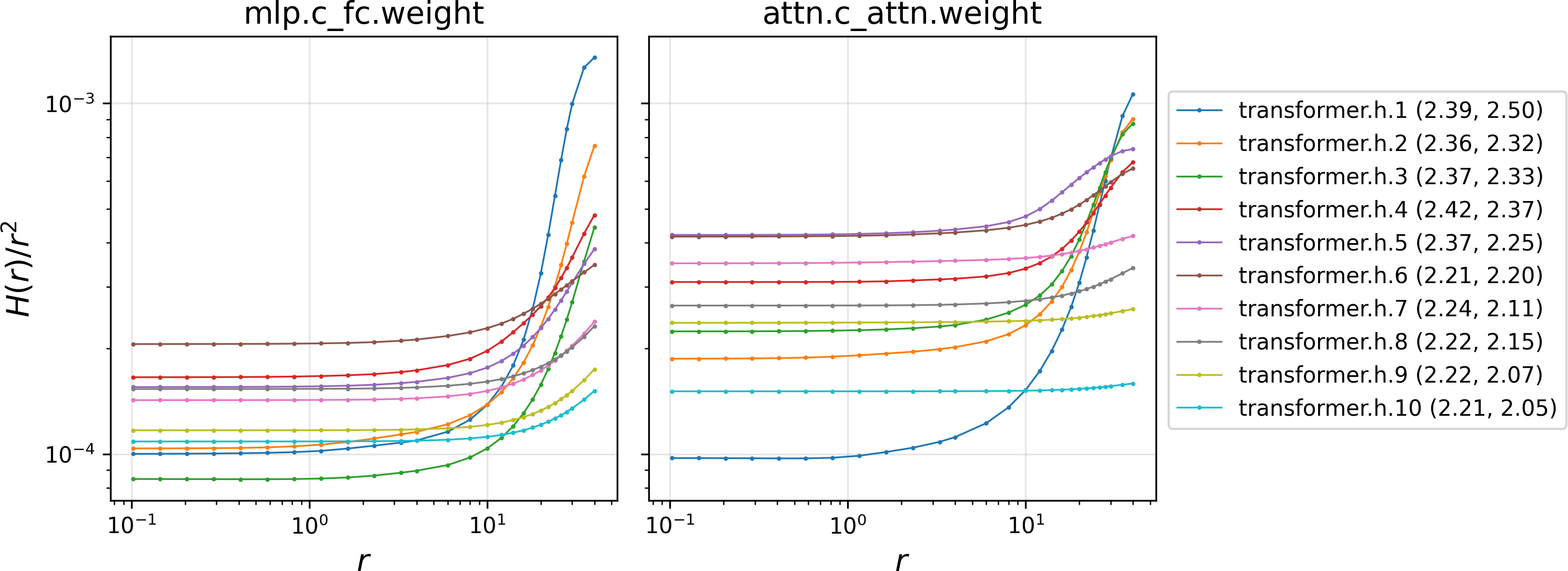
The model represents all the complex higher-order effects with a single function H(r), where r is the size of the step in any direction. Experiments show H tends to grow faster than a simple square law as steps get larger. That means big steps get penalized increasingly, which affects the best shape of the update.
What did they find?
1) Keep the same directions, change the strengths
The optimal update matrix should align its directions with the gradient’s directions. In other words, you keep the gradient’s singular spaces (its special axes), but you are allowed to change how strong each axis is (the singular values). This supports the idea of using the matrix structure, not flattening weights into a vector.
Why this matters: If you ignore the matrix structure, you might rotate the update into worse directions. Keeping the same directions but adjusting their strengths is both simpler and better.
2) Make the strengths more similar (spectrum homogenization)
Under realistic curvature growth (H grows faster than quadratic), the best update makes the singular values more even. If one direction is much stronger than another, the model prefers to reduce that imbalance. This “homogenization” improves conditioning, which usually makes optimization more stable and efficient.
Why this matters: Muon sets all singular values equal (perfectly uniform). The model says the right thing is to move toward more uniform values—but not necessarily all the way to identical. So Muon is directionally correct, but may be overly aggressive.
3) Full orthogonalization is optimal only in an extreme case
If the curvature function H has a “kink”—its growth rate suddenly jumps from slow to very fast—then making all singular values equal (full orthogonalization) becomes the optimal move. This explains when and why Muon’s full orthogonalization can be best.
Why this matters: In practice, curvature probably doesn’t jump that sharply. So full orthogonalization is a great extreme-case strategy, but the truly optimal update might keep the singular values close, not exactly equal.
Why are these results important?
- They give a clear, simple reason to respect matrix structure during training, instead of flattening everything like Adam does.
- They explain why methods like Muon work: they push toward better-conditioned updates by balancing directions more evenly.
- They also suggest Muon’s approach might be improved by making the singular values “more equal” rather than “exactly equal,” depending on how the curvature behaves for the task and model size.
Implications and potential impact
- Better optimizers: The isotropic curvature model is a convex program (which is easier to analyze and often easier to solve). It hints we can design new, practical optimizers that:
- Estimate how curvature grows with step size,
- Then choose an update that keeps the gradient’s directions but adjusts singular values to the best levels.
- Efficiency and stability: Making singular values more similar can improve conditioning, potentially reducing training time and making very large models more stable to train.
- Theory guiding practice: Instead of trial and error, this framework offers a principled way to tune “how much” orthogonalization to apply, based on measured curvature growth in the model.
Takeaway
Think of training as steering a spaceship down a valley. The gradient tells you where the valley slopes downward. But the valley’s walls curve differently depending on how far you move. This paper shows that for giant models, a smart captain keeps the ship pointed in the same useful directions, but evens out the engines’ power across those directions. If the valley’s walls suddenly get super steep beyond a certain distance, then making all engines equally powerful (full orthogonalization) is the best move—Muon’s strategy. Otherwise, slightly uneven but more balanced engines can be even better.
Knowledge Gaps
Knowledge gaps, limitations, and open questions
Below is a focused list of what remains uncertain or unexplored in the paper, framed to guide actionable future research.
- Empirical validity of the isotropy assumptions:
- Do curvature spectra and higher-order terms truly exhibit isotropy across directions and layers in modern LLMs?
- How large are anisotropy effects over the course of training (early vs. late), across architectures (attention vs. MLP), and under different data regimes?
- Dropped dependence on the base point:
- The model ignores the dependence of curvature on the current activations (the term’s dependence on Wu_i). How strongly does actual curvature vary with the base input Wu_i, and how does this affect optimal updates?
- Input distribution simplification:
- The assumption u_i ∼ i.i.d. uniform sphere is unrealistic; actual u_i have structured covariances. How do conclusions change under elliptical or data-driven distributions for u_i?
- Curvature function specification and estimation:
- The curvature function H(·) is left unspecified beyond monotonicity/convexity. How can H be estimated online efficiently and robustly per layer, with acceptable overhead?
- How stable is H across training steps and mini-batches, and how quickly must it be re-estimated?
- Growth model fidelity and plateau behavior:
- The super-quadratic growth model (H(r) ≈ c r{2+α}) is based on GPT-2 small. Does the exponent α and the growth-to-plateau transition generalize to larger LLMs, different tasks, or training phases?
- At what radius r does H(r) begin to plateau in practice, and how should this inform step-size bounds or trust regions?
- Convexity requirement and scope:
- The analysis requires H(√x) convex. Under what realistic training conditions (architectures, data distributions, regularization) does this hold, and where does it break?
- Multi-step dynamics and optimizer components:
- The model is single-step and omits momentum, EMA of gradients, weight decay, clipping, and schedule effects. How do these components interact with spectrum homogenization over multiple steps?
- Rectangular cases and dimensional constraints:
- Results and proofs assume m ≥ n for exact orthogonalization. What are precise characterizations and implementable rules when m < n, and how close to optimal can we get?
- Robustness to isotropy violations:
- How sensitive are the homogenization and alignment results to moderate anisotropy in curvature or data? Can we design robust variants that degrade gracefully?
- Algorithmic gap: computing Q⋆ efficiently:
- The paper does not provide a scalable GPU-friendly algorithm to solve the convex program for Q⋆ while preserving singular vector alignment and monotone spectral mapping. Can we develop such solvers that match Muon’s efficiency?
- Monotone spectral transforms:
- Polynomial approximations (e.g., Newton–Schultz) are generally non-monotone and can reorder singular values. How can we construct fast monotone spectral transforms that implement the optimal homogenization dictated by H?
- Quantifying optimal homogenization:
- Beyond “more homogeneous,” can we derive closed-form or numerically efficient mappings σ → σ⋆ that depend on the empirical H and dimension, and provide tuning rules for how much to homogenize?
- Learning-rate and scale selection:
- The model is scale-invariant and does not prescribe the magnitude of σ⋆ or step-size c. How should c be selected jointly with spectrum homogenization to optimize loss reduction and stability?
- Orthogonalization kink condition:
- Orthogonalization is shown optimal only under a sharp “kink” (jump) in H′. What quantitative bounds on A and B (the subdifferential interval) make orthogonalization optimal in finite dimensions, and how can we test for this condition in practice?
- Generalization impact:
- Does spectrum homogenization (or orthogonalization) improve generalization, calibration, or robustness, beyond training speed? Can we connect homogenization strength to downstream performance metrics?
- Error bounds for the surrogate model:
- What are tight bounds on the gap between the surrogate objective and the true one-step loss change (including the neglected Wu_i dependence and stochasticity), and when are predictions reliable?
- Layer-wise coupling and network interactions:
- The analysis treats one matrix W in isolation. How do interactions with LayerNorm, residual connections, attention mechanisms, and cross-layer couplings affect the optimal Q across the whole network?
- Stochastic gradient effects:
- How does mini-batch noise and gradient variance interact with spectrum homogenization? Does homogenization reduce variance or bias in updates meaningfully?
- Degenerate and repeated singular values:
- The alignment proposition has caveats under repeated singular values. How can practical algorithms handle degeneracy to ensure stable alignment and ordering without performance loss?
- Constraints and regularization:
- How should weight decay, trust-region constraints, gradient clipping, or norm constraints be incorporated into the convex model, and what changes do they induce in the optimal spectrum?
- Practical estimation protocols for H:
- What probing strategies (e.g., low-rank directional tests) can estimate H(·) accurately online with minimal overhead, and how many probes are needed to stabilize the estimate?
- Extension to tensors and non-matrix parameters:
- Many parameters (e.g., convolutional kernels, attention tensors) have higher-order structure. How does the model extend to tensors, and do its conclusions (alignment, homogenization) still hold?
- Predictive power for Muon variants:
- Can the model predict when Muon, PolarGrad, or other matrix-gradient methods will outperform AdamW, and by how much, based on measured H and gradient spectra?
- Formal uniqueness and optimality conditions:
- Under what precise conditions is Q⋆ unique, and when does strict homogenization (vs. orthogonalization) become necessary? Can we characterize the full optimality landscape under realistic H?
- Large-scale empirical validation:
- The paper’s empirical support is limited (GPT-2 small). Systematic studies across scales (billions of parameters), datasets, and training phases are needed to validate the model’s assumptions and prescriptions.
Practical Applications
Immediate Applications
Below are practical, deployable ways to use the paper’s findings and methods across industry, academia, policy, and daily life.
- Spectrum-homogenized gradient updates in existing optimizers (software/AI infrastructure)
- Use case: Replace full orthogonalization (Muon/PolarGrad) with “soft orthogonalization” that applies a monotone, spectrum-smoothing transform to gradient singular values while preserving singular spaces.
- Tools/products/workflows:
- A PyTorch/JAX plugin that wraps Muon to apply a monotone map to singular values (e.g., cubic-root or clipped-linear transforms) using polynomial/power-iteration SVD approximations.
- Layer-wise toggles: apply stronger homogenization in layers where m ≥ n and gradients are full-rank, weaker elsewhere.
- Assumptions/dependencies:
- Isotropic curvature conditions hold sufficiently; H(r) exhibits super-quadratic growth and no extreme kink.
- Efficient approximate polar/SVD kernels are available on GPUs; overheads are acceptable relative to training step time.
- Empirical curvature auditing to tune optimizers (industry, academia)
- Use case: Measure the curvature function H(r) per layer to calibrate the degree of homogenization vs orthogonalization.
- Tools/products/workflows:
- A “Curvature Audit” micro-batch routine that computes H(r)/r2 curves (as in the paper’s GPT‑2 experiment) for select radii and layers during warm-up.
- A scheduler that sets homogenization strength based on detected power-law exponents (α > 0 implies stronger homogenization).
- Assumptions/dependencies:
- Curvature isotropy and i.i.d. directional sampling approximate reality at scale.
- Short audit windows do not destabilize training; audit compute is budgeted.
- Singular-space preservation checks in training pipelines (software/ML ops)
- Use case: Add a diagnostic to ensure update matrices preserve gradient singular spaces, in line with the isotropic curvature model’s optimality conditions.
- Tools/products/workflows:
- A training hook that compares the update’s left/right singular vectors to those of the gradient (using randomized SVD on submatrices).
- Alerting when polynomial approximations (Newton–Schulz, Chebyshev) drift singular-space alignment.
- Assumptions/dependencies:
- Randomized SVD is accurate enough; extra overhead fits training budgets.
- Layer-wise optimizer selection and guardrails (industry LLM training)
- Use case: Adopt Muon/PolarGrad for layers with measured super-quadratic H(r) growth and m ≥ n; fall back to AdamW/Shampoo or weaker homogenization where isotropy is suspect.
- Tools/products/workflows:
- A per-layer optimizer map, updated from curvature audits.
- Guardrails that cap homogenization for layers showing plateauing H(r) or non-isotropic behavior.
- Assumptions/dependencies:
- Reliable per-layer curvature signals; layer shapes (m, n) known and stable; gradients not rank-deficient.
- Hyperparameter guidance for spectrum-aware updates (industry, academia)
- Use case: Set learning rates and homogenization intensity according to measured α and the spread of gradient singular values.
- Tools/products/workflows:
- Rule-of-thumb: stronger homogenization when singular-value ratio spread is high and H(√x) is convex; smaller step sizes when α is large.
- Automated LR/beta schedules tied to curvature growth phases.
- Assumptions/dependencies:
- Convexity of H(√x) for the relevant magnitude range; stability under changing data distributions.
- Cost and energy reduction via matrix-gradient methods (industry, policy, daily life)
- Use case: Migrate large-model training from AdamW to spectrum-aware matrix-gradient methods (e.g., Muon), leveraging empirically supported FLOP reductions.
- Tools/products/workflows:
- Policy guidance for “Green AI” procurement: prefer spectrum-aware optimizers in RFPs; track energy per token during pretraining.
- Assumptions/dependencies:
- Hardware supports polynomial/polar approximations efficiently; reported FLOP improvements generalize across tasks and scales.
- Academic benchmarking of homogenization degrees (academia)
- Use case: Establish standardized benchmarks to compare orthogonalization vs graded homogenization across tasks.
- Tools/products/workflows:
- Shared benchmark suites, analysis notebooks, and open datasets to measure loss reduction per step, stability, and generalization.
- Assumptions/dependencies:
- Community consensus on metrics; reproducibility across frameworks.
Long-Term Applications
Below are applications that require further research, scaling, or development before broad deployment.
- Optimizer that solves the isotropic curvature convex program per step (software/AI infrastructure)
- Use case: New “Isotropic Optimizer” that estimates H online and directly solves min_Q −Tr(QGᵀ) + E[H(∥Qζ∥)] for Q, producing theoretically optimal spectrum transformations.
- Tools/products/workflows:
- Stochastic solvers (proximal/variance-reduced) that approximate the expectation over sphere directions.
- Online curvature estimators that fit H(r) (piecewise power-law) per layer.
- Assumptions/dependencies:
- Fast, stable solvers at scale; accurate H estimation without prohibitive overhead; convergence guarantees under nonstationary data.
- Auto-preconditioning meta-optimizers leveraging curvature isotropy (software/AI infrastructure)
- Use case: A meta-optimizer that continually infers curvature properties and adjusts spectrum transforms, step sizes, and layer-wise strategies automatically.
- Tools/products/workflows:
- Reinforcement learning or bandit controllers that balance homogenization strength vs stability; cross-layer coordination.
- Assumptions/dependencies:
- Persistent isotropic trends in high-order terms; robust online estimation; safe exploration policies during training.
- Hardware co-design for matrix-gradient methods (semiconductors, systems)
- Use case: GPU/TPU kernels specialized for polar decomposition, randomized SVD, and monotone singular-value transforms with minimal memory traffic.
- Tools/products/workflows:
- ISA extensions for spectrum-aware operations; kernel fusion for gradient → spectrum → update pipelines.
- Assumptions/dependencies:
- Vendor adoption; clear performance benefits vs standard kernels; compatibility with mixed precision and large batch regimes.
- Standardized curvature measurement and reporting (policy, academia)
- Use case: Protocols to report per-layer H(r) profiles, α exponents, and spectrum spreads as part of model cards and energy disclosures.
- Tools/products/workflows:
- “Curvature & Energy” reporting standards; compliance audits; funding agency requirements for large training runs.
- Assumptions/dependencies:
- Community agreement; toolchain integration; legal and privacy considerations.
- Architecture design that favors isotropy and m ≥ n where helpful (software, robotics, healthcare, finance)
- Use case: Modify layer shapes or introduce structures that make spectrum-aware updates more effective (e.g., scaled-orthonormal columns, balanced projection layers).
- Tools/products/workflows:
- Design patterns that stabilize singular-space alignment; training curricula that encourage homogeneous gradient spectra.
- Assumptions/dependencies:
- Task performance not degraded by architectural bias; compatibility with attention/mechanisms; careful ablations required.
- Theoretical extensions and guarantees beyond isotropy (academia)
- Use case: Generalize the model to non-isotropic data regimes, residual connections, and realistic Hessian correlations; obtain finite-sample and nonconvex guarantees.
- Tools/products/workflows:
- New analytical tools for spectrum evolution under stochastic gradients; refined models of H’s plateauing behavior.
- Assumptions/dependencies:
- Access to large-scale empirical datasets; collaboration across theory and systems teams.
- Broader societal and daily-life impacts via cheaper, greener training
- Use case: As spectrum-aware methods mature, lower-cost, lower-energy training yields more accessible AI services (education, healthcare triage, financial assistance bots), especially in resource-constrained settings.
- Tools/products/workflows:
- Edge-friendly models trained with spectrum-aware optimizers; sustainability certifications that prioritize such methods.
- Assumptions/dependencies:
- Cost and energy savings translate into lower consumer prices; infrastructure supports deployment at the edge.
- Curriculum and workforce upskilling in matrix-gradient optimization (education)
- Use case: Integrate spectrum-aware optimization and curvature auditing into ML courses and practitioner training.
- Tools/products/workflows:
- Teaching modules, labs replicating H(r) auditing, and projects on implementing monotone spectrum transforms.
- Assumptions/dependencies:
- Availability of open-source tooling; educator adoption; updates to certification standards.
Glossary
- Adam: An adaptive optimization algorithm that computes per-parameter learning rates using estimates of first and second moments of gradients. "If asked before 2025 which optimization method is used for training deep learning and LLMs, most practitioners would have answered Adam \cite{kingma2015}."
- AdamW: A variant of Adam that decouples weight decay from the gradient-based update to improve regularization. "AdamW \cite{loshchilov2019decoupled}, a popular variant of Adam,"
- Auto-preconditioned methods: Optimization approaches that implicitly adapt preconditioning from problem structure without explicit Hessian computation. "it could pave the way for a large class of auto-preconditioned methods."
- Chain rule for subdifferentials: A rule extending the chain rule to non-smooth convex functions, describing subdifferential of a composition. "By the chain rule for subdifferentials,"
- Compact SVD: The singular value decomposition that uses only the nonzero singular values and corresponding singular vectors. "let be the (compact) singular value decomposition (SVD);"
- Conditioning (of a matrix): A measure of numerical stability based on the ratio of largest to smallest singular values; better conditioning improves optimization stability. "which in particular improves the conditioning of the update matrix."
- Convex cone: A set closed under nonnegative linear combinations, important in convex analysis and optimization. "Clearly, is a convex cone in the positive orthant ."
- Convex optimization program: An optimization problem with a convex objective (and possibly convex constraints) guaranteeing global optima. "This model is a convex optimization program amenable to analysis,"
- Cross-entropy loss: A standard loss function for classification that measures the difference between predicted and true distributions. " is a (cross-entropy) loss function,"
- Curvature function : A scalar function modeling average higher-order (curvature) effects as a function of perturbation norm. "we introduce a curvature function such that ."
- Expectation over the unit sphere: Averaging a quantity with the input vector uniformly distributed on the unit sphere. "we assume for simplicity that is sampled from the unit sphere in ."
- First-order optimality condition: A necessary condition for optimality in convex problems based on gradient or subgradient inclusion. "The first-order optimality condition requires that be an element of the subdifferential of the term $\E_{\zeta \sim \text{sphere}} H(\|Q \zeta\|)$."
- FLOPs: Floating-point operations; a measure of computational cost in training models. "require only about 52\% of the FLOPs to achieve the same empirical performance as AdamW"
- Frobenius inner product: The matrix inner product equal to the sum of element-wise products or the trace of . "where denotes the Frobenius inner product."
- Gradient orthogonalization: Replacing the gradient by its unitary polar factor (with equal singular values) to form the update direction. "the gradient orthogonalization employed in Muon and other related methods is directionally correct but may not be strictly optimal."
- Growth condition (on curvature): An assumption on how fast the curvature function increases with perturbation size. "under a general growth condition on the curvature,"
- Hessian: The matrix of second-order partial derivatives of a function, encoding local curvature. "including the second-order Hessian and higher-order terms,"
- Hessian integral: A weighted average of Hessians along a line segment in input space. "the singular spaces of the Hessian integral "
- Isotropic curvature model: The proposed surrogate convex program assuming rotationally uniform curvature to model one-step optimization. "hence, we call it the isotropic curvature model."
- Isotropy (of curvature): The assumption that curvature is directionally uniform (rotationally invariant). "by assuming isotropy of curvature, including the second-order Hessian and higher-order terms, of the loss function across all perturbation directions; hence, we call it the isotropic curvature model."
- Kink (in curvature): A point where the derivative of the curvature function jumps, indicating a sharp change in growth rate. "we assume there is a kink at some radius , such that is small while is large."
- Matrix-gradient methods: Optimizers that respect the matrix structure of weights and gradients instead of vectorizing them. "to analyze the recently introduced Muon optimizer and other matrix-gradient methods for training LLMs."
- Mini-batch: A subset of the training data used to compute a stochastic gradient at each iteration. "The gradient on a mini-batch of training samples, denoted ,"
- msgn(): The unitary (polar) factor of a matrix used as an update direction in orthogonalized gradient methods. "the update direction , often denoted $\msgn(G)$,"
- Newton–Schultz iteration: A polynomial iterative scheme for approximating matrix inverses or polar factors efficiently on GPUs. "polynomial approximations, such as the Newton--Schultz iteration \cite{jordan2024muon},"
- Orthogonal matrices: Square matrices whose columns (and rows) are orthonormal, representing rotations/reflections that preserve norms. "for two orthogonal matrices and ,"
- Orthogonalization: Making singular values equal and using the unitary polar factor as the update direction. "orthogonalization is optimal in this asymptotic limit."
- Orthonormal columns: Columns that are mutually orthogonal and of unit length, preserving norms in their spanned subspace. "since and the columns of $\msgn(G)$ are orthonormal."
- Phase transition (in growth): An abrupt change in the growth behavior of a function, here applied to curvature growth. "when the curvature exhibits a phase transition in growth."
- Polar decomposition: Factorization of a matrix into a unitary (or orthogonal) part and a positive semidefinite part. "the unitary part from the polar decomposition of the gradient "
- PolarGrad: An optimizer variant that explicitly uses the polar decomposition connection in its design. "a variant of Muon was therefore named PolarGrad to better reflect its connection to classical numerical linear algebra"
- Power law: Functional growth of the form ; used to model super-quadratic curvature. "we may assume a power law "
- Rotationally invariant: Invariance of a model or objective under orthogonal transformations, reflecting isotropy. "The isotropic curvature model is rotationally invariant in the following sense:"
- Separating hyperplane theorem: A result guaranteeing the existence of a hyperplane that separates disjoint convex sets. "Next, we apply the separating hyperplane theorem to , which is closed, convex, and compact, and , which is closed and convex."
- Singular spaces: The left and right subspaces spanned by the singular vectors in an SVD. "such that the singular spaces of and are aligned."
- Singular value decomposition (SVD): Matrix factorization into orthogonal/unitary factors and a diagonal matrix of singular values. "let be the (compact) singular value decomposition (SVD);"
- Spectral distribution: The distribution of eigenvalues/singular values of a matrix or operator. "we impose the isotropy assumption that the spectral distribution depends on the perturbation only through its Euclidean norm ."
- Spectral norm perspective: An analytical focus on the operator 2-norm (largest singular value) to understand algorithms. "much of which adopts a spectral norm perspective"
- Spectrum homogenization: Making the singular values of an update more uniform while preserving their ordering. "a property we refer to as spectrum homogenization."
- Stochastic gradient: A noisy gradient estimate computed from a mini-batch rather than the full dataset. "which in practice is a stochastic gradient from a mini-batch."
- Subdifferential: The set of subgradients of a convex (possibly non-differentiable) function at a point. "the subdifferential of at is the interval ."
- Unitary matrix: A complex-valued analogue of an orthogonal matrix that preserves inner products; in the real case, orthogonal. "the unitary part from the polar decomposition of the gradient "
- Von Neumann's trace inequality: An inequality bounding the trace of a product of matrices by the sum of products of ordered singular values. "Lemma [von Neumann's trace inequality]"
Collections
Sign up for free to add this paper to one or more collections.

