Optimal Scaling Needs Optimal Norm
Abstract: Despite recent progress in optimal hyperparameter transfer under model and dataset scaling, no unifying explanatory principle has been established. Using the Scion optimizer, we discover that joint optimal scaling across model and dataset sizes is governed by a single invariant: the operator norm of the output layer. Across models with up to 1.3B parameters trained on up to 138B tokens, the optimal learning rate/batch size pair $(\eta{\ast}, B{\ast})$ consistently has the same operator norm value - a phenomenon we term norm transfer. This constant norm condition is necessary but not sufficient: while for each dataset size, multiple $(\eta, B)$ reach the optimal norm, only a unique $(\eta{\ast}, B{\ast})$ achieves the best loss. As a sufficient condition, we provide the first measurement of $(\eta{\ast}, B{\ast})$ scaling with dataset size for Scion, and find that the scaling rules are consistent with those of the Adam optimizer. Tuning per-layer-group learning rates also improves model performance, with the output layer being the most sensitive and hidden layers benefiting from lower learning rates. We provide practical insights on norm-guided optimal scaling and release our Distributed Scion (Disco) implementation with logs from over two thousand runs to support research on LLM training dynamics at scale.
Paper Prompts
Sign up for free to create and run prompts on this paper using GPT-5.
Top Community Prompts
Explain it Like I'm 14
Overview
This paper looks at how to set training settings (like learning rate and batch size) when you make a LLM bigger or train it on more data. The authors find a simple, surprising rule: the “strength” of the last layer of the model (measured by a special kind of size called an operator norm) stays about the same at the best settings, no matter how big the model or dataset gets. They call this “norm transfer.” They also measure how the best learning rate and batch size change with dataset size and share practical tips for better training.
Key Questions
The paper asks three main questions in everyday terms:
- Is there a simple signal we can watch during training that tells us when our settings are “just right” even as we scale up models and data?
- How should the best learning rate and batch size change when we train on more tokens (more data)?
- Do different parts of the model need different learning rates, and if so, what works best?
Methods and Approach
To answer these questions, the authors trained many versions of a Llama-style LLM:
- Think of a model like a big calculator made of layers. “Width” is how many units are in each layer (like more lanes on a highway), and “depth” is how many layers there are (more floors in a building).
- Learning rate is the size of each step the model takes while learning.
- Batch size is how many examples the model looks at before taking a step.
- Dataset size (measured in tokens) is how much text the model reads during training.
They used an optimizer called Scion, which is a training rule that reshapes the gradients (the directions of change) so certain layer “sizes” (norms) are controlled. They focused on the last layer (the output layer), which is like the final decision-maker that maps hidden features to words.
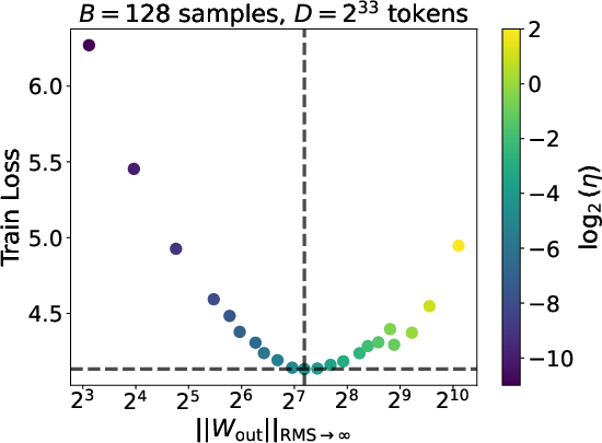
What’s an “operator norm”? Imagine each layer as a machine that takes in a vector and outputs another vector. The operator norm is like the maximum “amplification” this machine can apply. For the output layer, it measures how strongly the model can push its final scores. The team tracked this norm during training and compared it to the training loss (how wrong the model is).
Their procedure in simple steps:
- Pick a model size and a dataset size (number of training tokens).
- Run many trainings with different learning rates and batch sizes.
- For each run, record the training loss and the output layer’s operator norm.
- Find the settings that give the lowest loss and note the norm value there.
- Repeat while scaling the dataset and the model’s width/depth.
- Fit curves to the data to measure clear scaling rules.
Main Findings and Why They Matter
Here are the main findings in plain language:
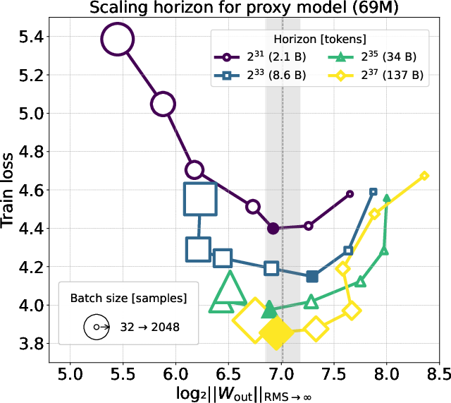
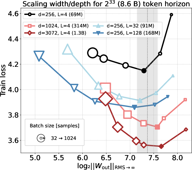
- Norm transfer (the big surprise): At the best settings (the lowest loss), the output layer’s operator norm is basically the same across different model sizes and different dataset sizes. In other words, even as you make the model wider or deeper, or feed it more text, the “sweet spot” keeps the output layer’s “strength” at about a constant level.
- Necessary but not enough: Many learning-rate/batch-size pairs can reach that same “right” norm value, but only one pair actually gives the best loss for a given dataset size. So hitting the right norm is required, but you still need the correct combo of learning rate and batch size to get the best performance.
- Clear scaling rules (what to set as data grows):
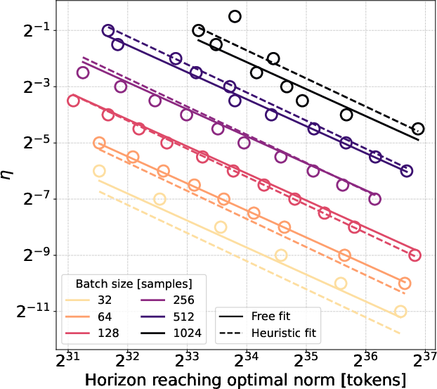
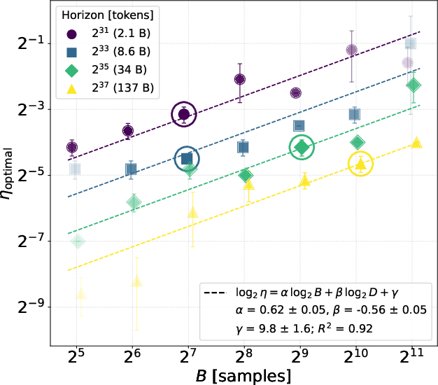
- Best learning rate grows with batch size roughly like η ∝ √B and shrinks with dataset size roughly like η ∝ D−0.56 (close to well-known “square-root” and “quarter-power” style rules from the popular Adam optimizer).
- The best batch size itself increases with dataset size roughly like B ∝ D0.45.
- Putting those together, the best learning rate for the best batch size behaves like η ∝ D−0.28.
Why this matters: It tells you how to set learning rate and batch size as you train on more data, reducing guesswork and saving compute.
- A practical trade-off: Around the best settings, there’s a “low-sensitivity” zone where performance doesn’t change much. Inside that zone, you can trade learning rate for batch size using the rule η ∝ √B, which can help you use bigger batches (often more efficient on large hardware) without hurting results.
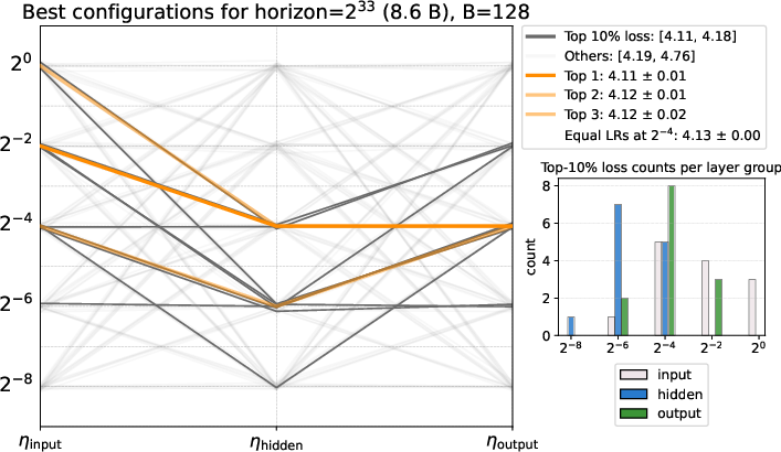
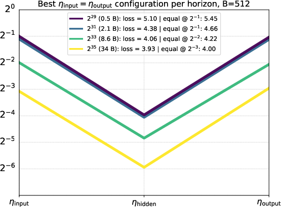
- Per-layer learning rates help: Giving the hidden layers a smaller learning rate than the input and output layers improved loss by up to about 6%. A simple, effective ratio that worked across datasets was:
- input : hidden : output = 1 : 1/8 : 1
- The output layer was the most sensitive to tuning, the hidden layers benefited from a lower rate, and the input layer was least sensitive.
- Tools and data: They released a distributed implementation of Scion (called Disco) and logs from over two thousand runs, so others can reproduce and study these training dynamics.
Implications and Potential Impact
- Easier scaling: Watching the output layer’s norm gives a simple, shared “compass” for tuning models as you make them bigger or train on more data. This can unify different tuning strategies and reduce costly trial-and-error.
- Practical recipes: The measured rules for learning rate and batch size give a clear starting point when planning large trainings. The per-layer learning-rate ratio (1 : 1/8 : 1) is a handy tip that consistently helps.
- Better use of hardware: The ability to trade learning rate and batch size in a safe zone means you can pick setups that use GPUs/TPUs efficiently without hurting accuracy.
- Open questions: Why does the constant-norm “sweet spot” exist? Is this special to Scion or more general? Could this constant-norm idea guide new optimizers or smarter training schedules? The paper opens doors for future research.
In short, the paper offers a simple rule of thumb—keep the output layer’s “strength” at a constant target—and backs it up with tested scaling laws and practical settings. This helps researchers and engineers train LLMs more confidently and efficiently.
Knowledge Gaps
Knowledge gaps, limitations, and open questions
Below is a concise list of what remains missing, uncertain, or unexplored, phrased so that future researchers can act on it:
- Theory for norm transfer: No theoretical explanation is provided for why a constant output-layer operator norm emerges as an invariant across model- and data-scaling. Formalize conditions under which training dynamics stay on a constant-norm manifold and characterize its geometry.
- Sufficiency beyond norm: The optimal norm is necessary but not sufficient; multiple (η, B) pairs reach the same norm with different losses. Identify additional measurable quantities (e.g., gradient-noise scale, curvature, Hessian spectrum) that disambiguate the unique optimal (η, B).
- Optimizer generality: Results are shown for Scion (with ablations for momentum/decay). Test whether the invariant norm and scaling exponents hold for Adam/AdamW (with EMA), SGD, Muon (with realistic EMA), and other norm-based optimizers.
- Regularization effects: Weight decay and spectral clipping are known to constrain norms, but their systematic impact on the invariant norm and scaling exponents is unquantified. Map how varying decay/clipping magnitudes shift the optimal norm and (η, B) scaling.
- Architectural dependence: The study uses a norm-everywhere Transformer with RMSNorm (no learned gains), specific residual/initialization choices, no biases, untied embeddings. Test robustness when using standard Pre-LN, LayerNorm with learned gains, alternative residual scalings (e.g., DeepNet/ReZero), tied embeddings, and bias terms.
- Dataset/domain breadth: Validate norm transfer and scaling rules across diverse corpora (code, multilingual, noisy web), different tokenizer/vocabulary sizes, mixture recipes, and data qualities.
- Training regime dependence: Findings are obtained in a non-repeating “infinite-data” setup. Replicate under finite-epoch, repeated sampling, curriculum schedules, and distribution shift to assess stability of the invariant norm and (η, B) rules.
- Scale limits: Experiments reach ~1.3B parameters and ~138B tokens. Confirm persistence (or breakdown) of the invariant and exponents at much larger scales (tens/hundreds of billions of parameters; >1T tokens), and check for surge/critical-batch phenomena at extreme batch sizes.
- Statistical rigor of fits: The optimal-norm and scaling exponents rely on curve-fitting of grid sweeps. Quantify sensitivity to grid resolution, fitting method, and seed variance; provide confidence intervals for the invariant norm value and exponents with independent replications.
- Single-run horizon evaluation: The “one long run” approach to probe multiple horizons may bias conclusions. Re-run each horizon independently (with fresh data order) to validate data-scaling exponents and the constant-norm target.
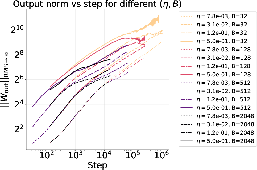
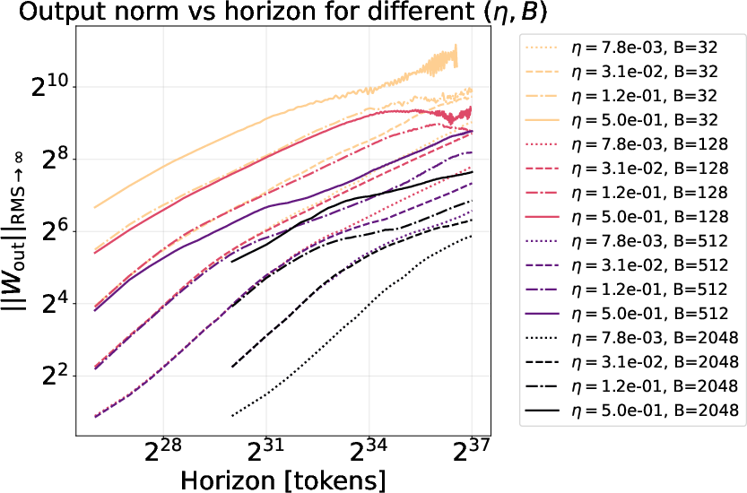
- Mechanism of piecewise norm growth: The observed piecewise-linear growth and “turbulence” region around 29–210 lack explanation. Analyze links to loss regimes, Hessian eigenvalue shifts, gradient-noise transitions, and optimization stability boundaries.
- Optimal batch-size cap: The claim of a horizon-dependent optimal batch size implies a cap on usable parallelism. Investigate methods to bypass this (e.g., noise injection, adaptive LR/BS scheduling, gradient accumulation strategies, curriculum) and provide a theory of the throughput–loss trade-off under norm constraints.
- Per-layer-group LR granularity: The proposed 1:1/8:1 input:hidden:output LR ratio was tested at coarse granularity. Explore finer splits (e.g., Q/K/V/O, MLP up/down, embeddings), block-wise schedules, and automated “mass tuning” driven by per-layer norm sensitivity.
- Output norm choice vs alternatives: While RMS→∞ (output) shows transfer (with some support for RMS→RMS and 1→RMS), a systematic search is missing. Identify which operator norms (per layer/group) are invariant across scales/optimizers, or whether a vector of per-layer norms forms the true invariant manifold.
- Positional encoding and sequence length: Results are for RoPE and context length 4096. Test different positional schemes (e.g., ALiBi, RoPE variants) and longer contexts to see whether the invariant norm value and scaling exponents shift.
- Measurement robustness and numerics: Operator-norm logging under mixed precision, sharding, and various parallelization strategies may introduce bias. Standardize numerically stable estimators, quantify precision error, and specify how norms are aggregated across shards.
- Dynamic control on-norm: The invariant suggests a control objective. Design and evaluate feedback controllers that adapt η and B online to keep the model on the constant-norm manifold; compare against static schedules for efficiency and stability.
- μP/depth-transfer connection: Depth scaling shows norm transfer without explicit depth-transfer tricks. Provide a formal link between Scion’s norm constraints, the chosen initialization/residual scaling, and μP-style transfer guarantees in depth.
- Link to square-root and quarter-power rules: Exponents (~0.62 for B, ~–0.56 for D) are close but not equal to 0.5 and –0.5. Derive exponents for Scion from SDE/mean-field analyses, explain deviations, and predict when surge or regime changes should occur.
- Generalization metrics: Training loss in infinite-data is used as a proxy for generalization. Validate on held-out validation perplexity, calibration, and downstream tasks to ensure the invariant norm and (η, B) scaling optimize generalization quality.
- Modalities and objectives: Extend to masked LM, instruction tuning, RLHF, ViTs, and multimodal models to test whether norm invariants and scaling rules persist beyond autoregressive LM pretraining.
- Learning-rate schedules and momentum: Ablations for LR decay and momentum are limited. Systematically map how warmup, cosine/linear decay, momentum magnitude/schedules alter the invariant norm target, sensitivity region, and optimal exponents.
- Vocabulary size sensitivity: Since the output layer maps to vocabulary, vary vocabulary size and tokenizer to test whether the numerical target of the RMS→∞ norm remains constant once properly normalized, or requires re-scaling.
- Why output layer is most sensitive: The output layer shows highest LR sensitivity. Investigate mechanisms (e.g., classifier margin, logit-norm theory, class-conditional row-norm dynamics) and whether targeted regularization can exploit this sensitivity.
- Hidden-layer norm invariants: The study centers on the output layer. Measure whether hidden-layer operator norms exhibit transferable targets across scales and whether joint constraints (multi-layer norm vectors) better predict optimality.
Practical Applications
Immediate Applications
The following applications can be deployed now, leveraging the paper’s findings, scaling rules, and released tooling. Each item includes sector relevance, potential tools/products/workflows, and key assumptions or dependencies.
- Norm-guided hyperparameter tuning (industry, software/ML infrastructure)
- Use case: Select learning rate and batch size using measured scaling rules to hit near-optimal loss without extensive sweeps.
- Tools/products/workflows:
- Implement a “norm-aware auto-tuner” that sets η and B using η(B,D) ∝ B0.62 * D-0.56, with B(D) ∝ D0.45 and η*(D) ∝ D-0.28.
- Start with small proxy runs to calibrate the constant factors for your stack; monitor the output layer operator norm during training to confirm the configuration is in the optimal region.
- Assumptions/dependencies:
- Most robust when using Scion (or closely related norm-based optimizers) and a “norm-everywhere” architecture (RMSNorm before each Linear).
- Observations were made on Llama 3–style Transformers, unconstrained Scion (no weight decay), and high-quality web-text data; momentum and LR decay preserved norm transfer in ablations.
- Optimal norm condition is necessary but not sufficient—still validate loss.
- Batch size/learning rate trade-offs for throughput (industry, cloud/HPC; academia)
- Use case: Increase throughput by moving within the low-sensitivity region around the optimal norm (η ∝ √B at fixed D), without degrading loss.
- Tools/products/workflows:
- “Throughput planner” that adjusts η and B jointly to maximize utilization subject to the acceptable loss band.
- Scheduling dashboards that visualize norm sensitivity and loss contour for informed trade-offs.
- Assumptions/dependencies:
- Requires knowing the token horizon D and monitoring output operator norm (RMS→∞) during training.
- Sensitivity depends on LR schedule; decay/momentum flatten sensitivity and widen acceptable regions.
- Device and batch-size planning from dataset size (industry, cloud/HPC ops; policy/compute governance)
- Use case: Select the number of accelerators given B*(D) ∝ D0.45 to avoid loss degradation or throughput inefficiency.
- Tools/products/workflows:
- Capacity planning tools that cap global batch size and map desired training duration (tokens) to optimal device counts and microbatch configurations.
- Procurement guidance that aligns cluster size with optimal batch size bands.
- Assumptions/dependencies:
- There is a practical upper bound on usable devices at a given horizon because B*(D) rises sublinearly in D.
- Verify for your optimizer and data distribution; weight decay or heavy regularization can change dynamics.
- Per-layer-group learning-rate layout for immediate loss gains (industry; academia)
- Use case: Improve training by reducing hidden-layer learning rate while keeping input/output rates equal; recommended ratio η_input : η_hidden : η_output = 1 : 1/8 : 1.
- Tools/products/workflows:
- Add a simple LR layout module to training configs; couple with norm monitoring to confirm stability.
- Combine with global η/B rules and adjust only the hidden group to reduce sensitivity.
- Assumptions/dependencies:
- Most validated with Scion and RMS→∞ norm on the output; uniform 1:1:1 is a strong baseline if multiple rates are cumbersome.
- Output layer is most sensitive; hidden is least—ensure correct grouping and optimizer hooks.
- Norm monitoring and guardrails (industry; software tooling; academia)
- Use case: Track output operator norm during training to detect divergence, turbulence regimes, or mistuning early.
- Tools/products/workflows:
- Lightweight “operator-norm dashboard” plugin for PyTorch/JAX training loops.
- Alerts when the norm drifts outside the optimal transfer band (~27 for the studied setup), or enters turbulence ranges (e.g., ~29–210).
- Assumptions/dependencies:
- Optimal target norm value depends on architecture/optimizer/dataset; calibrate once with proxy runs.
- Weight decay or spectral clipping constrain norms; thresholds should be adapted accordingly.
- Adopt Distributed Scion (Disco) in training pipelines (industry, cloud/HPC; academia)
- Use case: Replace or complement Adam/Muon with Scion via Disco to gain performance and insights with minimal overhead.
- Tools/products/workflows:
- Integrate Disco (FSDP/DDP/TP/EP/CP/PP compatible) with torchtitan; use released runs/logs to benchmark and reproduce scaling behavior.
- Assumptions/dependencies:
- Requires PyTorch/torchtitan compatibility and training-stack integration; verify licensing and infra constraints.
- Performance and scaling rules have been validated up to ~1.3B parameters and ~138B tokens.
- Training-budget and timeline estimation (industry; policy; academia)
- Use case: Estimate tokens-to-train, expected loss, and compute needs using η(D), B(D) rules and norm transfer for more predictable planning.
- Tools/products/workflows:
- “Budget calculator” that plugs scaling laws into cost models (GPU-hours, energy).
- Assumptions/dependencies:
- Calibrate constants per stack; cross-check with short pilot runs; consider data quality and pretokenization overheads.
Long-Term Applications
These applications require further research, scaling, standardization, or engineering to reach maturity.
- Real-time norm-controlled training controllers (industry; software tooling; academia)
- Vision: Closed-loop control systems that adjust η, B, momentum, decay, and clipping based on live operator-norm feedback to track the constant-norm manifold and avoid turbulence regimes.
- Potential products:
- “Norm autopilot” services integrated in cloud training platforms with SLAs for stability and efficiency.
- Dependencies:
- Robust norm estimation at scale; generalized targets across architectures/optimizers; safe policies for rapid adjustments.
- Generalization beyond LLMs to multimodal, vision, speech, and robotics (industry; robotics; healthcare)
- Vision: Apply norm transfer and scaling rules to other architectures, using appropriate operator norms (e.g., convolutional, attention variants) and layer groupings.
- Potential products/workflows:
- Norm-aware training recipes for medical imaging models or robot policy networks to improve stability and reduce tuning.
- Dependencies:
- Empirical verification across tasks; careful selection of “natural” norms for non-text modalities; domain-specific initialization and normalization.
- Hyperparameter transfer standards via “norm cards” (policy; academia; industry)
- Vision: Standardize reporting of operator norms and sensitivity bands in published models and datasets, enabling reproducible hyperparameter transfer across scales and institutions.
- Potential products/workflows:
- Documentation templates and benchmarking suites (e.g., on W&B HuggingFace) that include norm trajectories and target bands.
- Dependencies:
- Community agreement on which norms to track; governance for disclosures; consistency across optimizers.
- Compute governance and sustainability optimization (policy; energy; industry)
- Vision: Use B*(D) and η*(D) laws to set cluster sizing, quotas, and carbon budgets; avoid waste from overprovisioning devices beyond optimal batch size.
- Potential products/workflows:
- “Green training planners” that integrate carbon intensity and cost with norm-aware optimality constraints.
- Dependencies:
- Reliable mapping from training configurations to energy/carbon; policy alignment; diverse datasets and model sizes.
- Automated cross-scale hyperparameter transfer (industry; software tooling; academia)
- Vision: One-click transfer of tuned hyperparameters from small proxy to large models in width and depth using norm invariants, reducing or eliminating large-scale sweeps.
- Potential products/workflows:
- “Auto-transfer” modules that detect architecture changes and re-derive η/B settings while locking to constant-norm manifolds.
- Dependencies:
- Robust depth-transfer behavior across residual designs; strong validation for different normalizations and initializations.
- New optimizer designs grounded in manifold/norm theory (academia; industry)
- Vision: Derive optimizers that explicitly maintain training on constant-norm manifolds, yielding principled scaling behavior and improved generalization.
- Potential products/workflows:
- “Manifold-aware” optimizers and spectral constraints implemented in mainstream frameworks.
- Dependencies:
- Theoretical advances connecting the observed square-root and quarter-power laws to norm geometry; efficient SVD-free norm proxies.
- On-device and edge fine-tuning guardrails (industry; daily life; mobile)
- Vision: Lightweight norm monitors and LR controllers to prevent divergence in consumer-facing fine-tuning workflows (e.g., personalization on phones).
- Potential products/workflows:
- Mobile SDKs offering norm-aware LR schedulers and safe batch-size caps during quick local fine-tunes.
- Dependencies:
- Efficient norm estimates on constrained hardware; simplified layer-group tuning (e.g., hidden LR reductions) with minimal UI/UX complexity.
- Education and training curricula on norm-based optimization (academia; industry)
- Vision: Incorporate operator-norm monitoring, norm-everywhere architectures, and scaling rules into ML courses and upskilling programs.
- Potential products/workflows:
- Lab assignments with Disco, norm dashboards, and scaling-law estimators.
- Dependencies:
- Teaching materials, open datasets, reproducible baselines; community adoption.
Notes on Core Assumptions and Dependencies Across Applications
- Optimizer and architecture: The strongest results are demonstrated under Scion with a norm-everywhere design (RMSNorm before all Linear layers). Momentum and LR decay maintain norm transfer but may alter sensitivity.
- Data and tasks: Experiments used Llama 3–style Transformers trained on Nemotron-CC partitions with causal LM; transfers to other domains need validation.
- Measurement regime: Many results come from constant LR schedules without warmup, in an infinite-data setting; practical adaptations (e.g., decay, weight decay, spectral clipping) should be calibrated.
- Scale validity: Findings were validated up to ~1.3B parameters and ~138B tokens; extrapolation to much larger scales is promising but should be empirically checked.
- Optimal norm as necessary (not sufficient): Matching the output operator norm to the optimal band is required for transfer, but does not guarantee minimal loss—use scaling rules and small pilot runs to pinpoint constants for your stack.
Glossary
- Adam optimizer: An adaptive gradient-based optimizer that uses first and second moment estimates; used as a baseline for scaling rules. "matching the known square-root scaling rules for the Adam optimizer."
- Big-Theta notation (Θ): Asymptotic notation indicating tight bounds on scaling behavior. "The symbol is employed following the 'Big-O' notation, indicating scaling behaviour (in this case, 'constant' ...)."
- Causal language modelling: Training objective where the model predicts the next token given past context. "All the models are pretrained with the causal language modelling task."
- Disco (Distributed Scion): A distributed implementation of the Scion/Muon optimizer for large-scale training. "we release Disco ... a distributed implementation of the Scion/Muon optimizer compatible with modern parallelization strategies"
- Duality maps: Norm-induced transformations of gradients that enforce bounded updates and steepest descent under a given norm. "derived duality maps, i.e.~transformation rules of the gradients induced by a given norm."
- Exponential Moving Average (EMA): A smoothed running average of parameters or gradients often used in optimizers. "only in the case with no exponential moving average does Adam coincide with the steepest descent in 'max-of-max norm'"
- FlashAttention-2: A fast, memory-efficient attention implementation for transformer models. "FlashAttention-2"
- FSDP/DDP/TP/EP/CP/PP strategies: Parallelization techniques (e.g., Fully Sharded Data Parallel, Distributed Data Parallel, Tensor/Expert/Context/Pipeline Parallel). "supports FSDP/DDP/TP/EP/CP/PP strategies"
- Horizon (token horizon): The dataset size measured in tokens over which performance and scaling are evaluated. "hereafter referred to as horizon , measured in tokens"
- Induced operator norm: The norm of a linear operator measured between two vector-space norms, defined as a maximized ratio of output to input norms. "the 'α to β' induced operator norm is given by:"
- Learning rate decay: A schedule that reduces the learning rate over training to stabilize or improve convergence. "The impact of learning rate decay is also important, as we find it greatly flattens the norm optimum"
- Llama 3 architecture: A specific LLM architecture used in experiments. "we use the Llama 3 architecture"
- Maximum Update Parametrization (µP): A parametrization ensuring feature learning at infinite width and enabling hyperparameter transfer across widths. " introduces theoretically grounded scaling rules for hyperparameters as a function of model width in order to ensure 'maximal' feature learning in the infinite width limit."
- Mean field theory: A theoretical framework used to analyze scaling behavior and optimizer dynamics in the infinite-width limit. "Theoretically, \citet{kexuefm-11285} explains this from the mean field theory perspective."
- Momentum buffer: Stored moving average(s) of gradients used by optimizers to accelerate convergence. "they require only one momentum buffer (compared to two for Adam)"
- Muon optimizer: A norm-based optimizer that applies RMS→RMS assumptions to hidden layers and often outperforms Adam at scale. "One prominent example of the norm-based view on model optimization is the Muon optimizer"
- Nemotron-CC dataset: A processed CommonCrawl-based corpus used for pretraining. "we use a high-quality partition of the Nemotron-CC dataset"
- Norm-based optimization: An approach that controls operator norms of weights and updates to guide training dynamics. "norm-based optimization ... reframes optimization as a process that controls the operator norms of the model's weight matrices and gradient updates."
- Norm-everywhere approach: A design ensuring inputs to all linear layers are normalized (typically by RMSNorm) throughout the model. "we employ a norm-everywhere approach, inspired by the concept of well-normedness"
- Norm sensitivity: The degree to which performance changes when deviating from the optimal operator norm. "We relate this to the notion of learning rate sensitivity ... that we rephrase as norm sensitivity."
- Norm transfer: The phenomenon where the optimal operator norm remains invariant across model and dataset scaling. "We refer to this phenomenon as norm transfer"
- Operator norm: The induced norm of a linear mapping (matrix) between normed spaces, capturing its maximum amplification. "the operator norm of the output layer"
- One-to-RMS operator norm (1→RMS): The operator norm mapping an ℓ1 input to RMS output; equal to the max RMS column norm. ""
- Output layer: The final linear projection to the vocabulary that is most sensitive to learning-rate tuning. "The output layer is invariant to both width and depth scaling"
- Pre-LN setup: Transformer variant applying layer normalization before sublayers (attention/MLP). "Effectively, this corresponds to Pre-LN setup with QK-norm plus three additional normalisation layers"
- QK-norm: Normalization applied to the query/key projections within attention. "Pre-LN setup with QK-norm"
- Residual scaling factors: Multiplicative factors applied to residual branches to stabilize deep models. "no residual scaling factors"
- RMS norm: The root-mean-square vector norm used to standardize representations. ""
- RMSNorm: A normalization layer that scales inputs to unit RMS without learnable parameters. "by a preceding RMSNorm layer without learnable parameters"
- RoPE (Rotary Positional Embedding): A positional encoding method that rotates query/key vectors to inject position. "RoPE with "
- RMS-to-RMS operator norm (RMS→RMS): The induced norm mapping RMS inputs to RMS outputs; tied to the spectral norm. ""
- RMS-to-infinity operator norm (RMS→∞): The induced norm mapping RMS inputs to ℓ∞ outputs; depends on max row RMS. ""
- Scion optimizer: A norm-centric optimizer that assigns operator norms per layer and transforms gradients via duality maps. "Using the Scion optimizer, we discover that joint optimal scaling across model and dataset sizes is governed by a single invariant: the operator norm of the output layer."
- Semi-orthogonal initialization: Weight initialization where matrices are (semi-)orthogonal to improve stability. "Semi-orthogonal initialization for hidden linear layers"
- Spectral clipping techniques: Methods that enforce bounds on spectral properties (e.g., Lipschitz) during training. "with various spectral clipping techniques"
- Spectral condition: Constraints on weight and update norms necessary for feature learning and transfer in the infinite-width limit. "the spectral condition specifies bounds on the norms of weights and weight updates that are necessary to ensure feature learning."
- Spectral norm: The largest singular value of a matrix, used to bound operator behavior. "where is the spectral norm, also equal to the largest singular value"
- Steepest descent (under a norm): The direction of fastest decrease in loss given a chosen norm geometry. "ensures the steepest descent under the chosen norm"
- Surge phenomenon: A hypothesized transition in learning-rate scaling with batch size at critical scale. "we observe no surge phenomenon"
- Singular Value Decomposition (SVD): Matrix factorization into singular vectors/values used in defining duality maps. "with singular value decomposition (SVD) "
- SwiGLU: An activation function variant used in transformers that gates via a Swish-like nonlinearity. "SwiGLU activation function"
- Torchtitan: A training framework used to orchestrate large-scale model training. "torchtitan training framework"
- Weight decay: L2 regularization on weights that constrains norm growth during optimization. "we use Scion without weight decay"
- Well-normedness: A design/property where model components are consistently normalized to improve stability. "inspired by the concept of well-normedness"
- Zero-shot hyperparameter transfer: The ability to reuse optimal hyperparameters across model sizes without retuning. "allowing for what is known as zero-shot hyperparameter transfer"
Collections
Sign up for free to add this paper to one or more collections.