Scaling Laws and Spectra of Shallow Neural Networks in the Feature Learning Regime
Abstract: Neural scaling laws underlie many of the recent advances in deep learning, yet their theoretical understanding remains largely confined to linear models. In this work, we present a systematic analysis of scaling laws for quadratic and diagonal neural networks in the feature learning regime. Leveraging connections with matrix compressed sensing and LASSO, we derive a detailed phase diagram for the scaling exponents of the excess risk as a function of sample complexity and weight decay. This analysis uncovers crossovers between distinct scaling regimes and plateau behaviors, mirroring phenomena widely reported in the empirical neural scaling literature. Furthermore, we establish a precise link between these regimes and the spectral properties of the trained network weights, which we characterize in detail. As a consequence, we provide a theoretical validation of recent empirical observations connecting the emergence of power-law tails in the weight spectrum with network generalization performance, yielding an interpretation from first principles.
Paper Prompts
Sign up for free to create and run prompts on this paper using GPT-5.
Top Community Prompts
Explain it Like I'm 14
1. What is this paper about?
This paper studies “scaling laws” for simple neural networks. A scaling law tells you how a model’s prediction error goes up or down when you change things like:
- how much data you have (n),
- how big the model is (number of features d),
- and how strong your regularization is (λ, a small “keep it simple” penalty during training).
The authors look at two very simple two-layer (shallow) networks in a setting where the network actually learns features (not just uses fixed ones). They explain, from first principles, when these networks learn well, when they overfit, and how the shapes of their learned weights (their “spectra”) relate to generalization performance.
2. What questions did the authors ask?
They asked:
- How does the prediction error scale as we change the number of training examples, the model size, and the strength of regularization?
- Why do we sometimes see “bottlenecks” (places where getting more data alone doesn’t help) and “double descent” (error goes down, then up, then down again)?
- What do the learned weights look like inside the model, and how do those shapes (the spectrum of eigenvalues) relate to overfitting or good generalization?
- Can we predict all of this accurately using a simple mathematical tool (AMP), even outside the usual settings where it’s proven to work?
3. How did they study it? Methods and ideas
To keep things clear, the authors analyze two very simple network types and connect them to well-known problems:
- Diagonal linear network → LASSO:
- Think of a network that first rescales each input by a learned weight and then adds them up.
- With weight decay (a “don’t grow weights too big” penalty), training this network turns out to be mathematically equivalent to LASSO, a classic method that picks only the important inputs by pushing many weights to exactly zero.
- Quadratic network → Low-rank matrix estimation (matrix compressed sensing):
- Here the activation is quadratic (it squares a certain linear combination), and the model can be described by a learned matrix S.
- With weight decay, training becomes equivalent to estimating a low-rank matrix using a “nuclear norm” penalty (like an L1 penalty but for matrices). This pushes many small singular values to zero and favors simple, low-rank structure.
Teacher–student setup:
- The data is made by a hidden “teacher” network (plus some noise).
- We train a “student” network and measure its extra prediction error compared to the best possible model (this is called “excess risk”).
Power-law targets:
- The teacher’s important features follow a power-law: a few features matter a lot, many matter a little.
- This is common in real life (for example, city sizes or word frequencies follow power laws).
Predicting outcomes:
- They use approximate message passing (AMP), a fast mathematical “calculator” that predicts what training will do without actually training.
- AMP gives “state evolution” equations that predict things like the error and the spectrum of learned weights.
- Although AMP is formally proven in certain limits, the authors test it widely and find it predicts well even outside those strict conditions.
A helpful definition:
- Effective sample size n_eff:
- For the diagonal network, n_eff = n.
- For the quadratic network, n_eff = n/d (because each example carries information about many matrix entries).
- Using n_eff lets them present unified results for both models.
4. What did they find, and why is it important?
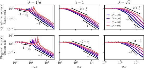
4.1 A “phase diagram” of scaling laws
As you vary data (n), model size (d), and regularization (λ), the error falls into clear regions (“phases”). Here’s the story in plain language:
- With too little data or too-strong regularization, the model can’t learn much: the error is stuck on a plateau (rank collapse).
- As you add data (and tune λ), the error starts to drop quickly because the model learns the strongest features first.
- If you keep adding data without enough regularization, the model may start fitting the noise (harmful overfitting). This can produce a peak in error near “interpolation” (where the model exactly fits the training data) — a version of the “double descent” curve.
- With even more data, the error drops again and can fall very fast.
Key takeaway:
- There is an optimal regularization level λ that avoids the harmful overfitting phase and achieves the best-possible (Bayes-optimal) error rates for these problems.
- For the quadratic network, the important axis is n_eff = n/d (not just n), explaining why widening a model changes how much data you effectively need.
4.2 The shape of learned weights (spectra) explains generalization
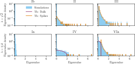
The authors show the learned weights look like a “noisy, soft-thresholded” version of the teacher’s weights:
- Soft-thresholding means: small values get pushed to zero; large values survive but are slightly shrunk.
- The learned spectrum typically has:
- A spike at zero (many exactly-zero values) — this is “rank collapse” when extreme.
- A “bulk” of small values near zero — often learned noise.
- A few large “spikes” far from zero — the important learned features.
Why this matters:
- Spikes = learned signal (good).
- Bulk = learned noise (bad if it gets too big).
- Zero spike = missed features (underfitting).
- Watching how these parts change as n and λ change tells you whether you are learning signal, noise, or both.
This gives a first-principles explanation for experimental findings in large neural networks, where heavy-tailed spectra and bulk-plus-spike shapes have been linked to generalization.
4.3 A simple, “universal” error breakdown
They split the error into three parts that match the spectrum:
- Underfitting: power in features you didn’t learn (spikes that stayed hidden or were cut to zero).
- Overfitting: power in the learned noise (the bulk near zero).
- Approximation: the learned features are not perfect (spikes shifted or shrunk by noise and regularization).
This decomposition works across cases and directly connects what you see in the spectrum to why the error is high or low.
4.4 Optimal regularization and pruning
- The best λ balances learning features while not learning noise. With the right λ, the error matches the best possible rates known in statistics for these problems.
- Because regularization mostly sets small eigenvalues to zero, a simple pruning rule (“cut small singular values to zero”) can achieve optimal error rates too. This supports why pruning works so well in practice.
4.5 AMP predictions work surprisingly well
- Even when used outside its fully proven regime, AMP’s predictions for error and spectra match simulations closely.
- This suggests AMP can be a practical tool for planning how to scale models and datasets.
5. Why does this matter? Implications and impact
- Smarter scaling: The phase diagram tells you when to add data, when to add regularization, and how model width changes how much data you effectively need (n_eff). This can save compute and guide training schedules.
- Read the spectrum: By looking at the learned weight spectrum, you can diagnose whether your model is learning signal, learning noise, or missing features — and fix it by tuning λ or pruning.
- Theory that matches practice: The paper gives a clear mathematical reason for patterns seen in real deep networks (like heavy-tailed spectra and double descent).
- Simple models, deep insights: Even shallow networks can teach us general lessons about feature learning that often carry over to deeper models.
- Practical tools: Regularization and pruning — already common tricks — are justified here as near-optimal strategies when used thoughtfully.
In short, the paper explains when and why small neural networks learn well or overfit, shows how their internal weight shapes tell that story, and provides a roadmap for tuning training to get the best results with the least waste.
Knowledge Gaps
Knowledge gaps, limitations, and open questions
The paper advances theory for scaling laws and learned spectra in shallow networks via mappings to LASSO and matrix compressed sensing, but it leaves several important aspects unresolved. Below is a concrete list of gaps and questions that future work could address:
- Rigorous non-asymptotic guarantees: Provide high-probability error bounds and explicit constants for the excess risk and spectral predictions beyond proportional asymptotics (arbitrary scalings of n, d, p, λ), and formally justify the heuristic extension of AMP/SE used throughout.
- Universality of AMP/SE: Establish conditions under which state evolution remains accurate outside Gaussian designs and fixed aspect ratios, including misspecified models, heavy-tailed noise, correlated features, or sub-exponential inputs.
- Data distributions beyond Gaussian: Analyze the impact of non-isotropic covariances, structured correlations, heavy-tailed or sub-Gaussian inputs, and real data (e.g., images, text) on both scaling laws and learned spectra.
- Noiseless targets and intermediate noise: Extend the phase diagrams and spectral characterizations to Δ = 0 and small-noise regimes, quantifying how overfitting phases, interpolation peaks, and rate transitions change without label noise.
- Activation functions beyond linear/quadratic: Generalize results to ReLU, piecewise-linear, and smooth nonlinearities; quantify whether the “bulk + spikes + bleed-out” phenomenology and rate exponents persist for other activations.
- Deeper architectures: Test whether the proposed universality (effective sample size, spectral phases, error decomposition) extends to multi-layer/deep networks, residual connections, and convolutional architectures.
- Width scaling and second-layer learning: Characterize how width p (and its scaling with d and n) affects n_eff, phases, and rates when second-layer weights are learned (not fixed all-ones), and quantify deviations for sublinear or superlinear widths.
- PSD constraint and nuclear norm: Clarify the role of the PSD constraint (S ≽ 0) in the quadratic mapping; for PSD matrices the nuclear norm equals the trace—does the regularizer effectively reduce to trace regularization, and do the phase diagrams change under this perspective?
- Mapping assumptions and robustness: Precisely state and test the conditions under which the diagonal-network/weight-decay ERM is equivalent to LASSO, and quadratic-network ERM to nuclear-norm minimization (e.g., presence of bias terms, scaling, normalization, and solver choice).
- Effect of optimizer and training dynamics: Investigate whether gradient descent/SGD (with finite steps, batch noise, momentum, and early stopping) reaches the ERM minimizer assumed here, and how optimization dynamics alter spectra and generalization relative to the ERM solution.
- Discontinuous phase boundaries: Quantify the constants and finite-sample behavior at rate discontinuities (e.g., λ ≍ √(n_eff/d), n_eff ≍ d), and test whether the observed jumps persist or smooth out in practical finite-d regimes.
- Effective sample size definition: Justify and generalize n_eff beyond the two studied models. How does n_eff depend on architecture, width p, activation, and learned layers in broader settings?
- Estimating δ and ε from data: Develop practical estimators for the effective noise (δ) and effective regularization (λε) that can be computed from a finite dataset to guide λ selection, pruning thresholds, and phase identification.
- Data-dependent regularization and model selection: Propose and analyze procedures (beyond cross-validation) that adapt λ to n, d, p, and target smoothness γ to avoid harmful overfitting while achieving near-Bayes-optimal rates.
- Target spectrum misspecification: Study robustness when the teacher’s spectrum is not exactly power-law, when γ is unknown or varying across layers, or when the target is not rotationally invariant (e.g., structured eigenvectors).
- Label/noise models: Extend analysis to non-Gaussian label noise (heavy-tailed, heteroskedastic, adversarial), input noise, and semi-supervised settings; quantify changes in phases and spectra.
- Error decomposition generality: Formalize the “universal” error decomposition (overfitting/underfitting/approximation) for architectures beyond quadratic and diagonal networks, and identify sufficient conditions for its validity.
- Spectral validations on real trained networks: Systematically test the predicted bulk/spike/bleed-out phases, heavy-tailed spectra, and interpolation peaks on modern deep networks trained on real tasks, controlling for confounders.
- Optimal pruning results: The pruning corollary is incomplete; fully specify the pruning rule, derive sharp conditions under which pruning achieves optimal rates, and compare to weight decay and early stopping in practice.
- Role of logarithmic factors: Remove or tighten “up to log factors” statements in the diagonal (LASSO) case; provide explicit logarithmic dependencies and their practical impact on λ selection and sample complexity.
- Second-layer heterogeneity: Analyze the effect of nonuniform second-layer weights in the teacher and student (beyond all-ones), including sign patterns and sparsity, on learned spectra and scaling behavior.
- Double descent geometry: Provide a quantitative description of the interpolation peak (height, width, location) in terms of δ, ε, γ, n, d, and λ, and connect it to spectral shape (bulk second moment) with explicit constants.
- Beyond nuclear/L1 norms: Explore other regularizers (group lasso, ℓp quasi-norms, spectral p-norms, path norms), their induced spectra, and the resulting phase diagrams and rates.
- Out-of-distribution generalization: Study how distribution shift affects the spectral phases and risk decomposition, and whether the learned spectra carry predictive power for OOD performance.
- Computational constraints and scaling: Analyze compute–data–model trade-offs explicitly (training time, memory, solver complexity), and connect them to the phase diagram to guide resource allocation.
- Practical λ calibration rules: Derive simple, implementable rules (e.g., λ ≍ √(n_eff/d)) with finite-sample corrections and uncertainty quantification, validated empirically across regimes.
- Measuring spectral components: Provide robust estimators for bulk size, spike counts, and bleed-out boundaries in finite d, along with statistical tests to classify phases from trained weights.
Practical Applications
Immediate Applications
The following applications can be deployed now by practitioners and researchers who train or analyze shallow neural networks, or who already use LASSO/matrix compressed sensing workflows. Each item notes sector links, potential tools/workflows, and key assumptions.
- Regularization rule-of-thumb for shallow networks to achieve near-optimal generalization
- Sector: software/ML, education
- What to do: use the paper’s optimal regularization scaling to set weight decay early in training:
- Define the effective sample size
n_eff:n_eff = nfor diagonal networks;n_eff = n/dfor quadratic networks. - Set
λ ≈ c * sqrt(n_eff/d)for some constantccalibrated on a small validation set. This sits near the optimal range identified in the phase diagram and avoids harmful overfitting. - Workflow: add a “λ scheduler” that initializes
λby the rule above and slightly tunescvia short validation sweeps. - Assumptions/dependencies: teacher-student or quasi-sparse targets with power-law spectra; weight decay is the main regularizer; shallow two-layer models; AMP predictions hold well in practice.
- Spectral monitoring to detect harmful overfitting and guide training decisions
- Sector: software/ML, reliability, healthcare (ML pipelines), finance (model risk), robotics
- What to do: monitor the spectrum of trained weights or layer-wise effective matrices during training. Watch for:
- Emergence of a large “bulk” near zero (learned noise) and reduction in spikes (learned features).
- Growth in the bulk’s second moment (signals entering Phase V/interpolation peak).
- Workflow: a “Spectral Dashboard” that computes approximate eigenvalue histograms for selected layers every few epochs; trigger increases in
λor early stopping when bulk grows. - Assumptions/dependencies: access to weight matrices; practical approximations for large layers using randomized SVD or sketches; generalization of spectral signals from these models to deeper architectures is heuristic.
- Post-training pruning via singular value thresholding
- Sector: software/ML, energy efficiency, robotics (edge deployment), mobile AI
- What to do: prune small singular values post-training by applying a threshold (soft-thresholding/Nuclear-norm-like) aligned with the learned cutoff:
- If
λwas small: prune the bulk near zero; ifλwas large: keep outliers and zero the rest. - Workflow: an “SVT Pruner” that runs after training, sets small singular values to zero, and revalidates. This is supported by the paper’s result that pruning mirrors optimal regularization effects.
- Assumptions/dependencies: matrices/layers where SVD is tractable or approximable; the spectrum-based pruning generalizes to deep nets empirically (formal guarantees shown for the quadratic/diagonal cases).
- Data acquisition ROI estimator based on scaling laws
- Sector: product/ML ops, policy within organizations, finance/healthcare model governance
- What to do: estimate marginal gains from adding more data vs increasing model size. Use the phase diagram and rates:
- In the quasi-sparse regime with
1 << n_eff << d^(2γ), expect risk ∼n_eff^(−1 + 1/(2γ)). - Past
n_eff ≳ d^(2γ), expect diminishing returns and transition to aΘ(d/n_eff)regime. - Workflow: build a dashboard that predicts expected error reduction curves as you vary data, width
d, andλ; prioritize balanced scaling to avoid harmful overfitting plateaus. - Assumptions/dependencies: power-law target; mapping of your architecture to the studied shallow regime is approximate; γ may need to be estimated from validation or spectral fits.
- LASSO-based feature selection with principled
λscaling- Sector: healthcare (omics, imaging-derived features), finance (tabular risk factors), social sciences (survey features)
- What to do: directly apply the LASSO equivalence of diagonal networks to perform feature selection under quasi-sparsity:
- Set
λ ∼ sqrt(n/d)(up to logs) for minimax rates in heavy-tailed targets. - Use the error decomposition to interpret which features are learned vs underfit.
- Workflow: integrate these
λscalings into AutoML/tabular pipelines; report spectral summary of learned coefficients (spikes vs bulk). - Assumptions/dependencies: features roughly quasi-sparse in some basis; i.i.d. noise approximations; convex LASSO; γ estimated or treated as a hyperparameter.
- Matrix compressed sensing guidance for low-rank estimation (e.g., imaging)
- Sector: healthcare (MRI/CT reconstruction), scientific imaging, recommendation systems
- What to do: apply nuclear-norm regularization with
λtuned asλ ≈ c * sqrt(n/d)(withn_eff = n/din the quadratic setting); monitor bulk to avoid learning noise. - Workflow: plug the
λrule into CS solvers; add spectral diagnostics to reconstruction pipelines to detect rank collapse or bulk growth. - Assumptions/dependencies: measurement operators reasonably close to rotationally invariant/GOE approximations; quasi-low-rank targets; noise behavior approximating Gaussian.
- Training workflows and educational modules
- Sector: academia, ML education
- What to do: use the provided code and phase diagram to teach scaling-law behaviors (plateaus, transitions, double descent); demonstrate spectral–generalization links in classroom labs.
- Workflow: Jupyter-based labs that vary
n,d,λ, visualize spectra, and compare to AMP-based state evolution predictions. - Assumptions/dependencies: shallow network examples; students can run small experiments; AMP predictions are used heuristically beyond formal regimes.
Long-Term Applications
These applications will benefit from further validation beyond shallow networks, non-Gaussian data, and idealized measurement assumptions. They may require new tooling, scaling, or theoretical extensions.
- Automated scaling planners for deep networks
- Sector: software/ML platforms
- Vision: a “Model Scaling Planner” that suggests how to jointly scale data, model width/depth, and regularization to hit target error under compute constraints, using generalized
n_eff, γ-estimation, and AMP-like predictors. - Dependencies: extension of phase diagrams to deep architectures; robust γ estimation from spectra; better non-asymptotic guarantees.
- Spectral-based generalization auditors for high-stakes ML
- Sector: healthcare, finance, autonomous systems
- Vision: a “Spectral Auditor” that continuously monitors bulk growth, bleed-out, and spike counts across layers, providing alerts when entering harmful overfitting regimes (Phase V), with suggested
λor early stopping adjustments. - Dependencies: scalable spectral approximations in large models; validated thresholds correlating with real-world generalization across domains.
- Standards and policy for sustainable, reliable AI scaling
- Sector: policy/regulation, corporate governance
- Vision: guidelines that require reporting of scaling curves, spectral diagnostics, and regularization schedules to prevent wasteful compute use and harmful overfitting in deployed models. Procurement rules that encourage balanced data–model–compute scaling plans.
- Dependencies: consensus on reporting formats; sector-specific validation; alignment with privacy and compliance constraints.
- Hardware–software co-design for in-the-loop spectral operations
- Sector: semiconductor, edge AI, robotics
- Vision: accelerators that support efficient approximate SVD/sketching and on-chip singular-value thresholding to enable real-time pruning and spectral monitoring during training/inference.
- Dependencies: hardware support for randomized linear algebra primitives; integration with training frameworks; energy/performance studies.
- Domain-adapted compressed sensing with spectral control
- Sector: medical imaging, seismic, astronomy
- Vision: incorporate spectral diagnostics and
λschedulers in CS systems with structured measurement operators; develop protocols that adaptively adjustλto avoid learning noise while maximizing rank recovery. - Dependencies: theoretical extensions beyond GOE/rotational invariance; domain-specific measurement models; clinical validation.
- Robust hyperparameter agents via AMP-inspired predictors
- Sector: AutoML, MLOps
- Vision: agents that learn to set
λ, width, and data collection policies using AMP/state-evolution-inspired meta-models trained on historical scaling outcomes. - Dependencies: broader datasets of scaling behaviors; improved non-asymptotic error controls; generalization to diverse architectures.
- Energy-efficient AI through routine spectral pruning and regularization schedules
- Sector: energy, sustainability, enterprise ML
- Vision: organization-wide policies to apply spectral pruning post-training and tune regularization to minimize harmful overfitting and compute waste, with estimated savings tracked via dashboards.
- Dependencies: cultural adoption; toolchain integration; measurement of downstream accuracy and energy impacts.
Cross-cutting assumptions and dependencies
- The paper’s guarantees are exact for the studied shallow architectures and rely on equivalences to LASSO and nuclear-norm matrix estimation; generalization to deep models is promising but not yet proven.
- Targets with power-law (quasi-sparse) spectra and Gaussian-like inputs/noise are idealized; real data may be heavy-tailed but correlated or structured (requires calibration).
- AMP/state-evolution predictions are shown empirically accurate beyond formal regimes “down to constants,” but non-asymptotic guarantees in broader settings remain an active area of research.
- Computing spectra for large models can be costly; practical deployment will need randomized SVD/sketching and selective layer monitoring.
- Estimating the tail index
γfrom data is necessary to apply precise rate predictions; robust methods forγestimation should be part of workflows.
Glossary
- Approximate Message Passing (AMP): An iterative algorithmic framework for high-dimensional inference in structured estimation problems, often analyzed via state evolution. "approximate message passing (AMP) and its state evolution (SE)"
- Bayes-optimal: Refers to performance or rates that match those of an ideal Bayesian estimator under the assumed data-generating model. "Bayes-optimal rates"
- Bayesian risk: The expected risk (error) under the posterior distribution given the data, often used as a gold standard for comparison. "Bayesian risk R_{\rm BO}(\mathcal D) = E[R(,)|\mathcal D]"
- Bleed-out: A spectral phenomenon where small signal spikes merge into the bulk part of the spectrum near its edge. "creating a {\it bleed-out} effect."
- Bulk (of the spectrum): The continuous, dense part of an eigenvalue distribution, as opposed to isolated spikes/outliers. "the bulk corresponds to learned noise"
- Diagonal neural network: A shallow network with diagonal first-layer weights enabling feature-wise scaling, often equivalent to a linear model with implicit regularization. "The first architecture is a diagonal neural network"
- Dirac mass: A distribution concentrated at a single point, representing a point mass in the spectrum. "represents a Dirac mass at $0$"
- Double descent: A non-monotonic risk phenomenon where error peaks near interpolation and then decreases with more data or parameters. "is reminiscent of the double descent behavior"
- Effective sample size: A normalized measure of the number of observations relevant for the model class, used to unify analyses across settings. "the effective sample size"
- Empirical risk minimization (ERM): The principle of fitting model parameters by minimizing the average loss on the training data. "empirical risk minimization (ERM) problem"
- Excess risk: The difference between the risk of a learned estimator and the optimal (target) risk, measuring generalization error beyond irreducible noise. "the excess risk achieved by empirical risk minimization"
- Feature learning regime: A training setting where network parameters adapt features (not just linear readouts), going beyond the lazy or kernel regimes. "in the feature learning regime"
- Gaussian orthogonal ensemble (GOE): A random matrix ensemble of symmetric matrices with Gaussian entries, used to model noise spectra. "We denote the Gaussian orthogonal ensemble as GOE(d)"
- Harmful overfitting: A regime where fitting the training data, including noise, leads to increased generalization error. "transition from {\it benign} to {\it harmful overfitting}"
- Heavy-tailed: Describing distributions with power-law decay, implying large probability of extreme values; used for signals or spectra. "heavy-tailed distribution"
- Kernel methods: A class of algorithms that use kernel functions to implicitly operate in high-dimensional feature spaces. "kernel methods"
- LASSO: An optimization method with ℓ1 penalty promoting sparsity in linear models. "the LASSO problem"
- Lazy regime: A learning regime where features remain essentially fixed and only the top (linear) layer is effectively trained. "lazy regime"
- Low-rank matrix estimation: Recovering a matrix with small rank from limited and noisy observations, often via convex surrogates. "low-rank matrix estimation"
- Matrix compressed sensing: The problem of recovering a structured (e.g., low-rank) matrix from few linear measurements, analogous to vector compressed sensing. "matrix compressed sensing (or low-rank matrix estimation)"
- Minimax rate: The optimal worst-case convergence rate achievable by any estimator over a given function class. "minimax rate"
- Neural scaling laws: Empirical or theoretical power-law relationships between performance and resources (data, model size, compute). "Neural scaling laws underlie many of the recent advances"
- Neural tangent kernels (NTK): A kernel describing the function space explored by infinitely wide neural networks trained by gradient descent in the lazy regime. "neural tangent kernels (NTK)"
- Nuclear norm: The sum of singular values of a matrix; a convex surrogate for rank used in regularization. "nuclear norm"
- Outliers (spectral): Isolated, large eigenvalues corresponding to learned signal components separate from the bulk. "II (Outliers)"
- Over-parameterized: Having more parameters than training samples or than needed to interpolate the data, often changing optimization landscapes. "over-parameterized two-layer network"
- Power-law spectrum: An eigenvalue or coefficient decay pattern where magnitudes follow a power law with index γ. "a power-law spectrum"
- Quasi-sparsity: A signal model where coefficients are not exactly sparse but decay according to a heavy-tailed law, enabling compressive recovery. "the notion of {\it quasi-sparsity}"
- Random features regime: A setting where features are fixed random projections and only the linear readout is trained. "random features regime"
- Ridge regression: Linear regression with ℓ2 regularization, often used as a baseline in high-dimensional generalization studies. "ridge regression"
- Soft-thresholding: A shrinkage operation that sets small coefficients to zero and reduces larger ones by a threshold, as in LASSO solutions. "soft-thresholding function"
- Spectral properties: Characteristics of the eigenvalue distribution (bulk, spikes) of trained weight matrices and their relation to generalization. "the spectral properties of the trained network weights"
- State evolution: Deterministic recursion describing the asymptotic dynamics or fixed points of AMP algorithms. "state evolution equations"
- Stiefel manifold: The set of orthonormal matrices with a fixed number of columns; optimization constraints can restrict weights to this manifold. "Stiefel manifold"
- Teacher-student setting: A modeling setup where data are generated by a “teacher” model of known form and learned by a “student.” "the teacher-student setting"
- Weight decay: ℓ2 regularization on parameters during training to control complexity and improve generalization. "weight decay"
- Wigner semi-circle law: The limiting eigenvalue distribution of certain random symmetric matrices, forming a semicircular density on a bounded interval. "Wigner semi-circle law"
- Source and capacity conditions: Classical assumptions in kernel learning characterizing target smoothness (source) and hypothesis class complexity (capacity). "source and capacity conditions"
Collections
Sign up for free to add this paper to one or more collections.