Towards a Physics Foundation Model
Abstract: Foundation models have revolutionized natural language processing through a ``train once, deploy anywhere'' paradigm, where a single pre-trained model adapts to countless downstream tasks without retraining. Access to a Physics Foundation Model (PFM) would be transformative -- democratizing access to high-fidelity simulations, accelerating scientific discovery, and eliminating the need for specialized solver development. Yet current physics-aware machine learning approaches remain fundamentally limited to single, narrow domains and require retraining for each new system. We present the General Physics Transformer (GPhyT), trained on 1.8 TB of diverse simulation data, that demonstrates foundation model capabilities are achievable for physics. Our key insight is that transformers can learn to infer governing dynamics from context, enabling a single model to simulate fluid-solid interactions, shock waves, thermal convection, and multi-phase dynamics without being told the underlying equations. GPhyT achieves three critical breakthroughs: (1) superior performance across multiple physics domains, outperforming specialized architectures by up to 29x, (2) zero-shot generalization to entirely unseen physical systems through in-context learning, and (3) stable long-term predictions through 50-timestep rollouts. By establishing that a single model can learn generalizable physical principles from data alone, this work opens the path toward a universal PFM that could transform computational science and engineering.
Paper Prompts
Sign up for free to create and run prompts on this paper using GPT-5.
Top Community Prompts
Explain it Like I'm 14
Overview
This paper tries to build a “one model for many physics problems,” similar to how big LLMs can handle many language tasks without retraining. The authors introduce the General Physics Transformer (GPhyT), a single AI model trained on a huge mix of physics simulations (about 1.8 terabytes of data). The big idea: given a short “clip” of how a system is changing (like a few frames of a video), the model learns the rules of the physics happening and predicts what comes next—without being told the exact equations.
The key questions
The paper focuses on three simple questions:
- Can one big model learn many different kinds of physics (like smooth flows, shock waves, and hot/cold convection) without being told which is which?
- Can it handle brand-new situations it never saw before (new boundary rules or even new kinds of physics) just by “reading” the recent history of the system?
- Can it make stable predictions far into the future, not just one step ahead?
How did they build and train the model?
Think of GPhyT as a very smart “video watcher” for physics:
- The input is like a short video clip of the system: several frames showing fields such as velocity, pressure, or temperature over space and time.
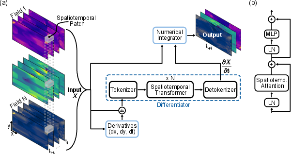
- The model chops this clip into small space–time blocks (like tiny 3D cubes: height × width × time). These are its “tokens,” similar to words in a sentence.
- A Transformer (the same core idea behind many LLMs) uses attention to look across all places and times at once. This helps it spot patterns like spinning vortices, sudden shock fronts, or heat plumes, no matter where they occur.
- It first learns the “rate of change” (how fast things are changing right now). Then a simple, classic numerical step (called Forward Euler) uses that rate to jump to the next frame. You can think of it like: if you know where something is and how fast it’s moving, you can guess where it will be a moment later.
To make the input clearer, the authors also feed in basic derivatives (quick, local measurements of how values change across space and time), which helps with sharp features like shock waves.
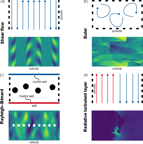
The training data covers many different types of physics:
- Smooth flows, obstacle flows around solid shapes, compressible flows with shock waves (Euler), and patterns from hot–cold convection (Rayleigh–Bénard).
- Even two-phase flow (like oil and water in porous material) and cases with heat moving between solids and fluids.
Two clever tricks push the model to learn general rules rather than memorize:
- Variable time gaps: the “video” can be sped up or slowed down, so the model must figure out the time scale from the context.
- Per-dataset normalization: each dataset is scaled differently, forcing the model to learn relative behavior (what matters physically) rather than absolute numbers.
What did they find?
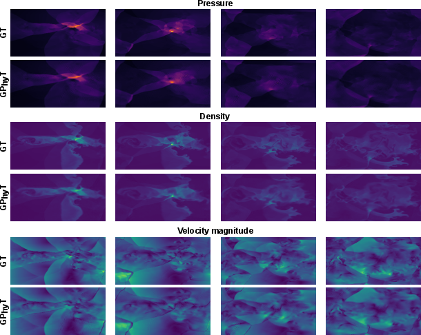
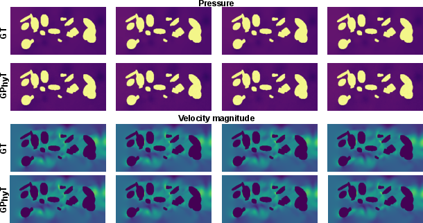
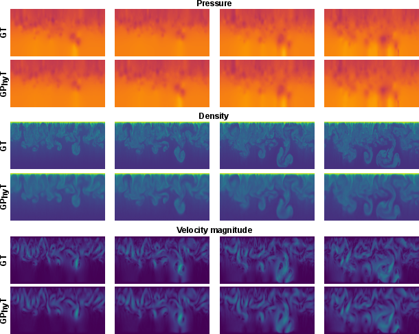
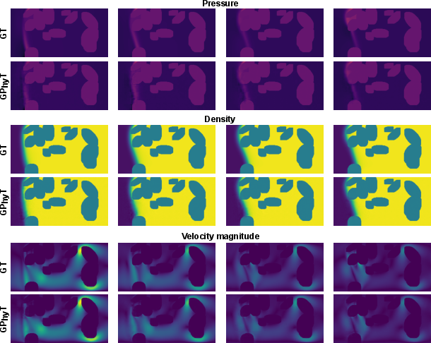
- One model works across many physics
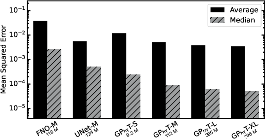
- GPhyT beat strong specialized methods (like UNet and Fourier Neural Operators) on average, often by large margins.
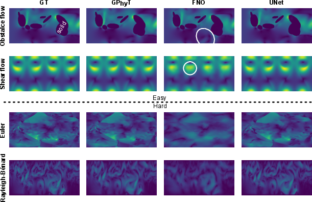
- It kept important details like sharp shock fronts and fine vortices better than the baselines.
- It scales well: bigger versions of the model generally performed better.
- Zero-shot generalization (works on new things without retraining)
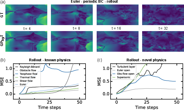
- New boundary rules: For example, the model trained with one kind of edge behavior (like wrapping around) could handle another (like open edges where stuff can flow out) just by seeing a short context. Its accuracy stayed close to the known cases.
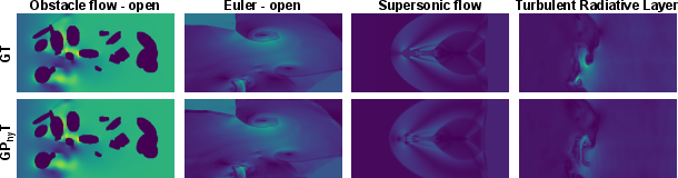
- New physics it never saw: It produced sensible, physically plausible predictions for supersonic flow around an obstacle (it formed the expected bow shock) and for a turbulent radiative layer. Errors were higher than for known systems, but the overall behavior looked right—impressive for zero training on those systems.
- Longer rollouts (predicting many steps ahead)
- Over 50 steps, the model kept global behavior stable and reasonable. Fine details gradually blurred (as expected), but big structures and trends stayed consistent.
- Error growth was near-linear for many cases, which is a good sign for stability. Harder cases (like two-phase flow) were tougher, as changes can happen very suddenly.
Why it matters and what’s next
If a single AI can “learn physics from context,” then:
- Scientists and engineers could simulate complex systems faster and more easily, without building a custom solver for each new problem.
- It could speed up research and design across fields: aerospace (shock waves), climate and weather (convection), energy systems (flows in porous media), and more.
- It helps “democratize” high-quality simulations—more people can access them without deep expertise or massive computing.
What still needs work:
- Extending to 3D, more types of physics beyond fluids, and handling different grid sizes and resolutions.
- Improving long-term stability so it stays accurate over very long predictions.
- Scaling up training data and model size may unlock even stronger generalization.
In short, this paper is an early but important step toward a universal “physics foundation model”: train once on diverse data, then adapt on the fly to many problems—just by looking at a short example of how the system is evolving.
Knowledge Gaps
Below is a concise, actionable list of knowledge gaps, limitations, and open questions that remain unresolved in the paper. Future work can use these to prioritize experiments, ablations, and extensions.
- Extension to 3D and complex meshes: The model is demonstrated on 2D, regular grids; it is unclear how to handle 3D domains, variable resolutions, adaptive meshes, or unstructured/curvilinear grids without retraining.
- Space–time attention scalability: The use of full spatiotemporal attention is computationally quadratic in token count; limits on resolution, sequence length, and memory are not quantified, nor are efficient variants (e.g., factorized/sparse attention) evaluated.
- Long-horizon stability and error control: Rollouts are shown up to 50 steps; behavior over much longer horizons, for stiff systems, or strongly chaotic regimes is unknown. No adaptive time stepping, CFL-aware constraints, or error-controlled integration strategies are explored.
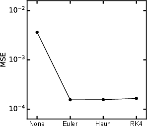
- Numerical integrator choice and learning: Only Forward Euler is used (with a brief ablation claim on RK4). It remains open how learned integrators, symplectic/energy-preserving schemes, or hybrid corrector steps affect stability and accuracy across physics.
- Physical-law satisfaction metrics: Evaluation is dominated by MSE. There is no systematic assessment of conservation (mass, momentum, energy), boundary condition satisfaction, shock location error, spectra/structure functions, or vorticity/energy budgets—especially during rollouts.
- Boundary condition coverage: Zero-shot tests consider periodic/symmetric/open BCs; moving/deforming boundaries, time-varying BCs, inflow transients, free surfaces, and multi-inlet/outlet networked domains are not studied.
- Real-world robustness and domain gap: All training/testing is on synthetic simulation data; robustness to measurement noise, partial observability, missing variables, sensor cadence, and calibration to experimental data is not evaluated.
- Absolute scale and unit calibration: Per-dataset normalization and inferring Δt from context preclude guarantees on absolute magnitudes/units. It is unclear how to explicitly condition on physical scales, dt outside the training range, or recover calibrated predictions across datasets.
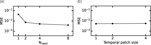
- Prompt length and ICL mechanics: The model uses 4-frame prompts, but there is no ablation on prompt length, many-shot behavior, or how context size and diversity affect in-context learning for different physics.
- Tokenization and positional encoding choices: Non-overlapping tubelets and absolute positional encodings are used; sensitivity to patch size, overlap, relative encodings, rotary embeddings, or multi-resolution tokenization is untested.
- Geometry representation and generalization: How obstacles/solids are encoded (e.g., masks, signed distance) and how the model generalizes to new, complex or CAD-derived geometries/topologies is not rigorously analyzed.
- Physics domain coverage: Training focuses on (mostly 2D) fluid-like systems (incompressible/compressible, convection, porous two-phase). There is no coverage of deformable solids/FSI with compliant structures, electromagnetics, combustion/chemistry, MHD, or radiative transfer beyond a qualitative “turbulent radiative layer.”
- Parameter conditioning and controllability: The model infers dynamics from fields alone; there is no mechanism to condition on physical parameters (Re, Ma, Pr, material properties) for controlled sweeps or design, nor an evaluation of parameter-token conditioning.
- Heterogeneous channel handling: Different datasets have different field sets; the approach to optional/missing channels, heterogeneous modalities, or adding new variables post hoc is unspecified.
- Multi-step baselines and fairness: Rollout comparisons against baselines (UNet/FNO) are not shown; it remains unknown whether improvements persist in multi-step settings and under identical training/evaluation protocols.
- Uncertainty quantification and OOD detection: The model provides point estimates only; predictive uncertainty, calibration, ensemble methods, and mechanisms to detect extrapolation or trigger fallbacks are absent.
- Data mixture design and scaling laws: There is no study of data-mixture weighting, curriculum across physics, or scaling laws (model/data/compute) for cross-physics generalization; data efficiency strategies (active learning, synthetic augmentation targeted to gaps) are unexplored.
- Train/test isolation and leakage: Given heavy sub-sampling and augmentations from trajectories, the paper does not detail safeguards to prevent trajectory-level leakage or temporal correlations crossing splits.
- Enforcement of constraints: While gradients dx, dy, dt are concatenated, there is no exploration of soft/hard constraint enforcement (e.g., divergence-free penalties, boundary masks, conservation constraints) and their effect on generalization.
- Solver coupling strategies: Interfaces for hybrid deployment (e.g., periodic corrections, residual learning over coarse solvers, mixed rollouts) are not proposed or evaluated for stability/accuracy trade-offs.
- Practical deployment costs: Inference latency, memory footprint on large domains, batching/tiling strategies, distributed inference, model compression/quantization/distillation, and real speedups versus high-fidelity solvers are not reported.
- Failure mode characterization: Beyond MSE increases in OOD cases, systematic diagnostics of where/why the model fails (e.g., shock overshoot, boundary layer thickening, energy drift) are not provided, nor are mitigation strategies (regularizers, curriculum, constraints).
- Licensing/reproducibility timing: Code, checkpoints, and extra datasets are promised but not yet released; reproducibility depends on future artifacts and detailed training logs/hyperparameters which are not fully specified.
Glossary
- Absolute positional encodings: Fixed position vectors added to tokens so a model can distinguish locations in sequences or grids. "Absolute positional encodings are added to the patches."
- Autoregressive rollout: Generating future states by repeatedly feeding a model’s own predictions back as inputs. "a 50-timestep autoregressive rollout"
- Boundary conditions: Constraints that specify behavior of a physical system at domain boundaries (e.g., walls, open inflow/outflow, periodicity). "a wide range of physical systems, boundary conditions, and initial states."
- Boundary layer: A thin region near a surface where viscous or diffusive effects dominate and gradients are high. "boundary layer dynamics"
- Bow shock: A curved shock wave formed ahead of an object moving supersonically through a fluid. "a bow shock wave"
- Central differences: A finite-difference scheme that approximates derivatives using values on both sides of a point. "using central differences."
- Compressible flow: Fluid motion where density changes are significant, often requiring the Euler or Navier–Stokes equations. "compressible (Euler) fluid dynamics"
- Computational fluid dynamics (CFD): Numerical simulation of fluid flows by solving governing equations on a computer. "computational fluid dynamics"
- DeepONet: A neural operator architecture that learns mappings from function spaces (operators), enabling PDE solution prediction. "DeepONets"
- Discretization-invariant: A property where a model’s performance does not depend on the specific mesh or grid resolution. "discretization-invariant"
- Discontinuities: Abrupt changes in field variables (e.g., at shock fronts) where derivatives are undefined. "discontinuities and chaotic dynamics"
- Euler shock waves: Shock phenomena governed by the inviscid compressible Euler equations. "Euler shock waves with periodic boundary conditions"
- Forward Euler method: A first-order explicit numerical integration scheme advancing a state using its current derivative. "Forward Euler method"
- Fourier Neural Operator (FNO): A neural operator using spectral (Fourier) layers to learn solution operators to PDEs. "Fourier Neural Operators (FNOs)"
- Governing equations: The differential equations (e.g., PDEs) that define the physics of a system. "new governing equations"
- In-context learning: Inferring tasks or dynamics from provided examples (prompts) without updating model weights. "in-context learning"
- Incompressible flow: Fluid motion where density is effectively constant and divergence of velocity is zero. "Incompressible flow with periodic boundary conditions"
- Inductive biases: Architectural or training assumptions that guide a model toward certain solution structures. "must incorporate inductive biases"
- Layer normalization (LayerNorm): A normalization technique applied across features within each token to stabilize training. "layer norms (LN)"
- Meta-learning: Learning to adapt quickly to new tasks or systems, often with few examples. "meta-learning"
- Neural differentiator: A learned module that predicts time derivatives of state variables for use by a numerical integrator. "The neural differentiator (blue dashed box)"
- Neural Operator (NO): A model class that learns operators mapping input functions to output functions, enabling PDE solution prediction. "Neural Operators (NOs)"
- Neural Ordinary Differential Equations (Neural ODEs): Models that parameterize the derivative of a system and integrate it to evolve states over time. "Neural ODEs"
- Numerical integrator: An algorithm that advances a system’s state over time given its derivative (e.g., Euler, Runge–Kutta). "numerical integrator"
- Physics-aware machine learning (PAML): ML methods that incorporate or exploit physical structure to model scientific systems. "physics-aware machine learning (PAML)"
- Physics Foundation Model (PFM): A large pre-trained model intended to generalize across diverse physics tasks without retraining. "Physics Foundation Model (PFM)"
- Physics-Informed Neural Networks (PINNs): Neural nets trained with physics constraints by embedding PDE residuals in the loss. "Physics-Informed Neural Networks (PINNs)"
- Porous media: Materials containing interconnected pores through which fluids can move, affecting flow and transport. "porous media"
- Rayleigh–Bénard convection: Buoyancy-driven convective flow in a fluid layer heated from below and cooled from above. "RayleighâBénard convection"
- Runge–Kutta 4: A classical fourth-order explicit time-integration scheme for ODEs. "RungeâKutta 4"
- Shock waves: Propagating discontinuities in pressure, density, and velocity in compressible flows. "shock waves"
- Spatiotemporal transformer: A transformer that attends jointly over space and time to capture dynamic physical patterns. "spatiotemporal transformer"
- Supersonic flow: Flow with speed exceeding the local speed of sound, typically featuring shock waves. "Supersonic flow around an obstacle"
- Tubelet tokens: Non-overlapping spatiotemporal patches used as tokens for transformer input in videos or 3D data. "tubelet"
- Turbulence: Chaotic, multi-scale fluid motion characterized by cascades of energy and complex vortical structures. "turbulence and shockwave interactions."
- Turbulent radiative layer: A turbulent flow regime influenced by radiative processes affecting momentum/energy transport. "turbulent radiative layer"
- Two-phase flow: Flow involving two distinct fluid phases (e.g., liquid–gas) interacting within the domain. "twophase flow"
- Vision Transformer (ViT): A transformer architecture for images that treats patches as tokens. "Vision Transformer (ViT)"
- Vortical structures: Coherent rotating flow features (vortices) central to many fluid dynamics phenomena. "vortical structures"
- Vortex shedding: Periodic release of vortices from bluff bodies in a flow, producing oscillatory wakes. "vortex shedding"
- Zero-shot generalization: Performing well on unseen tasks or systems without additional training. "zero-shot generalization"
Collections
Sign up for free to add this paper to one or more collections.