Precise Dynamics of Diagonal Linear Networks: A Unifying Analysis by Dynamical Mean-Field Theory
Abstract: Diagonal linear networks (DLNs) are a tractable model that captures several nontrivial behaviors in neural network training, such as initialization-dependent solutions and incremental learning. These phenomena are typically studied in isolation, leaving the overall dynamics insufficiently understood. In this work, we present a unified analysis of various phenomena in the gradient flow dynamics of DLNs. Using Dynamical Mean-Field Theory (DMFT), we derive a low-dimensional effective process that captures the asymptotic gradient flow dynamics in high dimensions. Analyzing this effective process yields new insights into DLN dynamics, including loss convergence rates and their trade-off with generalization, and systematically reproduces many of the previously observed phenomena. These findings deepen our understanding of DLNs and demonstrate the effectiveness of the DMFT approach in analyzing high-dimensional learning dynamics of neural networks.
Paper Prompts
Sign up for free to create and run prompts on this paper using GPT-5.
Top Community Prompts
Explain it Like I'm 14
A simple guide to “Precise Dynamics of Diagonal Linear Networks: A Unifying Analysis by Dynamical Mean-Field Theory”
1) What is this paper about?
This paper studies how a very simple kind of neural network learns over time, and why it sometimes learns fast but doesn’t generalize well (doesn’t do well on new data), and other times learns slowly but ends up generalizing better. The network is called a diagonal linear network (DLN). Even though it represents a simple linear function in the end, the way it is trained makes its learning behavior surprisingly rich.
The authors use a tool from physics, called Dynamical Mean-Field Theory (DMFT), to turn a complicated, high-dimensional training process into a small set of equations that are much easier to study. With these equations, they explain several puzzling training behaviors within one unified story and show a trade-off between learning speed and final quality.
2) What are the key questions?
The paper focuses on two big, easy-to-understand questions:
- How does the learning behavior change over time, especially depending on how big or small the starting weights are (the initialization)?
- What kind of solution does the network end up with after a long time, and how quickly does it get there?
3) How did they study it? (Methods explained simply)
- What is a DLN? Imagine you want to predict a number from many input features (like height, age, etc.). A standard linear model uses one weight per feature. A DLN uses two numbers per feature, u and v, and combines them in a special way so the effective weight becomes w = (u² − v²)/2. This makes the final function still linear, but the learning dynamics (how u and v change during training) are nonlinear and interesting.
- What is training here? They use “gradient flow,” which you can think of as continuous-time gradient descent: you keep nudging the parameters in the direction that reduces the training error. Sometimes they also add regularization (a small penalty on large parameters) to encourage simpler solutions.
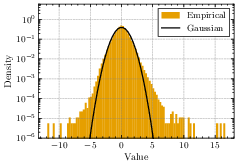
- What is DMFT? Picture trying to describe a crowd: tracking every person is too hard, but you can often describe the whole crowd’s behavior with a few simple numbers (like average speed). DMFT does something similar: it converts the huge, messy learning dynamics of many parameters into a single “effective” process that represents a typical parameter’s behavior. This yields low-dimensional equations that predict training error, test error, and how fast things change.
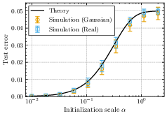
- Did they check it works? Yes. They:
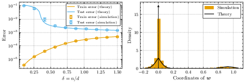
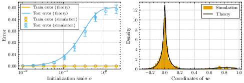
- Compared the theory’s predictions with computer simulations on random (Gaussian) and real datasets.
- Gave a rigorous justification for a closely related, slightly “smoothed” version of the DLN (so the math is well-behaved), supporting the overall approach.
4) What did they find, and why does it matter?
Here are the main discoveries, organized for clarity:
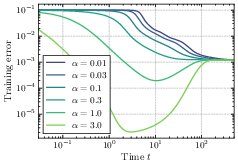
- Different learning phases show up depending on the initialization size (how big the starting weights are):
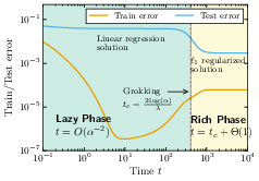
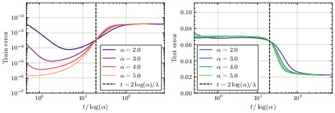
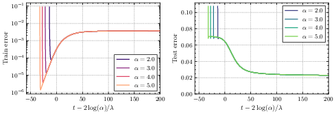
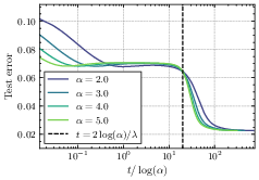
- Large initialization (start big):
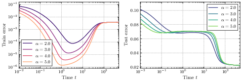
- Lazy phase: The network first behaves like a plain linear model. It reduces training error quickly but often generalizes poorly (it may memorize too much).
- Rich phase: Later, it switches sharply to learning sparser, simpler solutions that generalize better. The switch happens around a time proportional to log(initialization size). This sudden improvement resembles “grokking,” where a model suddenly starts to generalize well after a long period of seeming not to.
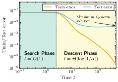
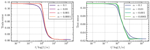
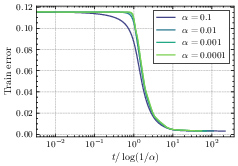
- Small initialization (start tiny):
- Search phase: Training barely changes at first (a plateau). The system is “deciding” which features matter.
- Descent phase: Then it starts improving, and it does so by “turning on” important features one by one (incremental learning). This phase unfolds on a timescale proportional to log(1/initialization size).
- What solution does training converge to?
- With regularization (λ > 0): It ends up behaving like L1-regularized regression, which tends to produce sparse solutions (most weights exactly zero).
- Without regularization (λ = 0):
- If you have more data than features (underparameterized), it converges to the usual least-squares solution.
- If you have more features than data (overparameterized), there are many exact-fit solutions. The training dynamics pick the one with the smallest value of a special “norm” that depends on the initialization size. Smaller initialization acts more like L1 (promoting sparsity), and larger initialization acts more like L2 (less sparse). That means small initialization tends to produce simpler, sparser models that often generalize better when the true signal is sparse.
- How fast does it converge?
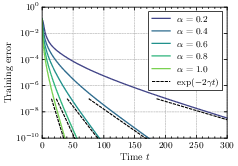
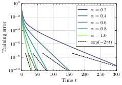
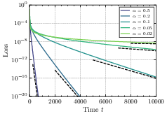
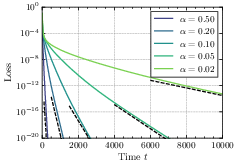
- With regularization, some parts of the model can converge very slowly, so the overall loss (error) may decrease sub-exponentially.
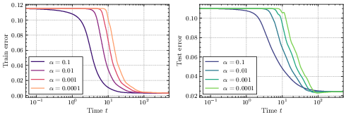
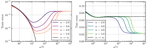
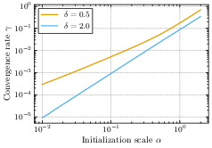
- Without regularization, the loss typically drops exponentially in time. However, the speed of this drop depends on the initialization size: smaller initialization makes convergence slower.
- Putting these together reveals a trade-off: smaller initialization often gives better final generalization (simpler solutions), but learning is slower; larger initialization learns faster but can overfit or generalize worse.
- Do the predictions match reality?
- Yes. Simulations with random and real-world data match the main predictions, including the phase structure (lazy/rich vs. search/descent), the sharp transition time scaling with log(initialization), the incremental learning pattern, and the speed–quality trade-off.
5) Why is this important?
This work gives a clear, unified picture of how even simple networks can show complex learning behavior. It shows that:
- The way you initialize a model matters a lot: small starts can lead to better, sparser final solutions but slower training. Large starts can learn fast early on but risk worse generalization.
- Sudden “grokking”-like improvements can come from a shift in the training phase and its implicit bias.
- DMFT is a powerful tool for understanding the learning dynamics of modern, high-dimensional models. This could guide better choices of hyperparameters (like initialization size and regularization) and smarter training schedules or early stopping rules.
- The idea that “better solutions are harder to find” (slower to reach) might be a general principle in these systems, with implications for how we budget training time and compute.
Overall, the paper connects several previously separate observations into one consistent framework, provides new predictions (like exact convergence rates on average), and offers both practical insights and mathematical tools that can be extended to more complex neural networks in the future.
Knowledge Gaps
The following points summarize the knowledge gaps, limitations, and open questions the paper leaves unresolved.
- Rigorous DMFT for the original DLN: Establish a full, non-truncated, rigorous derivation of the DMFT characterization for diagonal linear networks trained by gradient flow, including conditions ensuring existence, uniqueness, and stability of the effective process for broad input distributions (beyond sub-Gaussian and truncation).
- Formal proofs of timescale separations: Provide rigorous (high-probability) proofs of the lazy–rich and search–descent phase separations, including the transition times t_c ≈ 2 log(α)/λ (large α) and t_c ≈ 2 log(1/α)/Δ (small α), for finite δ and without relying on singular perturbation heuristics.
- Quantifying “grokking” sharpness: Precisely characterize and prove the sharpness of the transition to generalization (e.g., convergence in O(1) time after a Θ(log α) delay), and delineate parameter regimes (α, λ, δ, σ2, P_*) under which grokking occurs or fails.
- Convergence-rate theory in the regularized case: Derive tight upper and lower bounds and, where possible, closed-form expressions for pathwise and averaged convergence rates when λ > 0, including how rates depend on λ, δ, σ2, and P_*; explain and quantify the “arbitrarily slow” paths that induce subexponential averages.
- Explicit γ in the unregularized case: Obtain closed-form or efficiently computable expressions for the exponential rate γ in common target distributions (e.g., Bernoulli–Gaussian sparsity), prove its monotonicity in α under general conditions, and quantify its dependence on δ and σ2 with non-Gaussian inputs.
- Discrete-time optimization effects: Extend the analysis from continuous-time gradient flow to discrete-time gradient descent and SGD (including step-size schedules, momentum, and adaptive methods), and characterize how discretization and gradient noise reshape implicit bias, timescales, and convergence rates.
- Beyond diagonal linear networks: Generalize the DMFT analysis and trade-off findings to deep linear networks, multi-layer diagonal models, nonlinear activations, and transformer-like architectures; determine which phenomena (incremental learning, grokking-like transitions, speed–generalization trade-offs) persist.
- Input structure and covariance: Analyze DLN dynamics and DMFT under non-isotropic, correlated, or structured feature distributions (e.g., spiked covariance models), and determine how covariance structure changes phase boundaries, fixed points, and convergence rates.
- Loss and noise generality: Extend results to classification losses (logistic/hinge) and non-Gaussian or heteroscedastic label noise; assess whether the implicit biases and timescale separations carry over and how they transform.
- Alternative regularizations: Study other penalties (e.g., ℓ1/ℓ2 on u or v, ℓ2 or ℓp directly on w, group sparsity) and derive the corresponding fixed points and timescale structures; characterize how J_α changes under different regularization schemes.
- Initialization heterogeneity: Analyze non-uniform or random-sign initializations (coordinate-dependent α, layer imbalance u(0) ≠ v(0)), and quantify their effects on implicit bias (the norm J_α), incremental learning order, and convergence speed.
- Non-asymptotic guarantees: Develop finite-sample, finite-d error and rate bounds (with dimension and sample-size dependence) that validate DMFT predictions, clarify required problem sizes, and provide confidence intervals for test/train metrics.
- Activation schedule in incremental learning: Predict the order and timing of coordinate activations in the small-α descent phase, linking them to the distribution of target magnitudes P_* and noise σ2; provide distributional results (e.g., activation time order statistics).
- Complete phase diagram: Produce a quantitative phase diagram of regimes (lazy, rich, search, descent) with explicit boundaries in (α, λ, δ, σ2, P_*), and formally derive the observed change in training-error monotonicity around α ≈ 0.3.
- Universality vs. real-data deviations: Systematically test and explain deviations observed on real datasets; extend theory (e.g., beyond sub-Gaussian universality) to heavy-tailed inputs, covariate shift, and feature dependencies, potentially via higher-order DMFT corrections.
- Solvers and reproducibility: Develop stable, scalable numerical methods to solve the DMFT equations for general P_* and δ, prove existence/uniqueness for the original (non-truncated) system, and release code to foster reproducible DMFT-based predictions.
- Compute-optimal stopping: Use DMFT to design compute-optimal early stopping policies that balance the documented speed–generalization trade-off; quantify the gains and provide operational guidelines for stopping time selection.
- Sparsity-aware generalization metrics: Go beyond MSE to measure support recovery and false discovery rates at the fixed point, especially in sparse regression, and relate these metrics to α and λ choices.
- Tail behavior of pathwise rates: Characterize the distributional tails of pathwise convergence rates (e.g., near-threshold Δ ≈ 0) that drive slow averages, and explore regularization or initialization strategies that mitigate these tails.
- Regimes where small α harms generalization: Identify target and noise regimes (e.g., dense P_* or large σ2) where the small-α bias toward sparsity degrades performance; provide thresholds and decision rules for choosing α.
- SGD DMFT rigor: Establish a rigorous DMFT (or related stochastic effective process) for DLNs under SGD, including the impact of gradient noise scale, batch size, and annealing schedules on implicit bias and timescales.
- Multi-output extensions: Analyze DLN dynamics for multi-output regression/classification, including cross-task interactions and whether incremental learning persists across outputs.
- Extreme aspect ratios: Investigate behavior in the small-sample regime (δ → 0) and the high-sample regime (δ → ∞) beyond simplified ODEs, providing precise statements for fixed points and rates, and clarifying transitions between regimes.
- σ2 dependence: Quantify how label noise variance affects transition times, phase boundaries, fixed points, and convergence rates; identify noise-robust training/regularization strategies within the DLN framework.
Collections
Sign up for free to add this paper to one or more collections.

