Introducing the $σ$-Cell: Unifying GARCH, Stochastic Fluctuations and Evolving Mechanisms in RNN-based Volatility Forecasting (2309.01565v1)

Published 4 Sep 2023 in q-fin.CP

Abstract: This paper introduces the $\sigma$-Cell, a novel Recurrent Neural Network (RNN) architecture for financial volatility modeling. Bridging traditional econometric approaches like GARCH with deep learning, the $\sigma$-Cell incorporates stochastic layers and time-varying parameters to capture dynamic volatility patterns. Our model serves as a generative network, approximating the conditional distribution of latent variables. We employ a log-likelihood-based loss function and a specialized activation function to enhance performance. Experimental results demonstrate superior forecasting accuracy compared to traditional GARCH and Stochastic Volatility models, making the next step in integrating domain knowledge with neural networks.

Summary

The paper introduces the σ-Cell, a novel RNN architecture that unifies GARCH dynamics with stochastic and evolving mechanisms for improved volatility forecasting.
It employs dynamic parameter adjustments and stochastic layers to capture fluctuating market conditions with performance metrics superior to traditional models.
Empirical evaluations on S&P 500 and BTCUSDT datasets demonstrate reduced RMSE, MAE, and NLL, indicating enhanced predictive accuracy and robust volatility modeling.

Introducing the $σ$ -Cell for Volatility Forecasting

The paper "Introducing the $σ$ -Cell: Unifying GARCH, Stochastic Fluctuations and Evolving Mechanisms in RNN-based Volatility Forecasting" (2309.01565) introduces a novel RNN architecture designed to enhance financial volatility modeling by integrating aspects of traditional econometric models, such as GARCH, with cutting-edge neural network techniques.

Architectural Overview

The $σ$ -Cell RNN architecture is built around the principle of capturing dynamic volatility patterns by bridging deterministic econometric models with stochastic and evolving mechanisms:

Hybrid RNN-GARCH Approach: The $σ$ -Cell incorporates the logic of GARCH models, utilizing time-varying parameters to assess volatility based on past data and latent processes. Unlike classic GARCH, which assumes fixed parameters, the $σ$ -Cell parameters evolve as functions of the input data.
Stochastic Layers: The architecture enriches traditional deterministic models by introducing stochastic layers, allowing it to capture fluctuating market dynamics more effectively.
Generative Network Modeling: The model approximates the conditional distribution of latent variables, employing a log-likelihood-based loss function and specialized activation functions to enhance predictive accuracy.
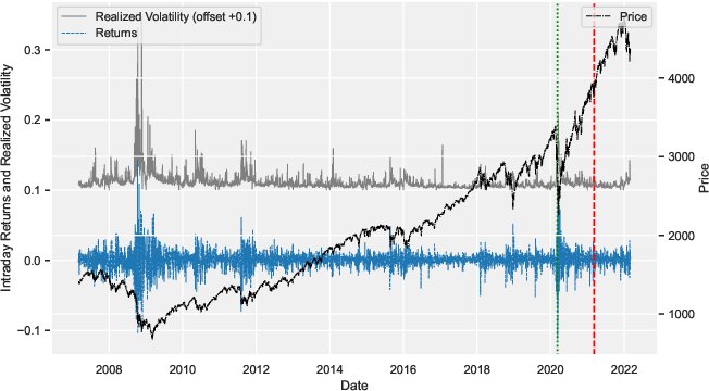
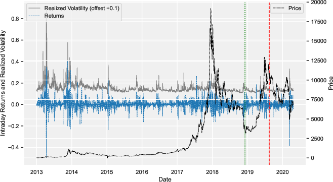
Figure 1: The following plot illustrates Realized Volatility, Returns, and Price of S{additional_guidance}P 500 Index over Time. This plot displays the realized volatility (RV, offset +0.1), intraday returns, and price of the S{additional_guidance}P 500 index from March 10, 2007, to March 1, 2022.

Implementation Details

Model Components

Dynamic Volatility Modeling:
- The volatility $\sigma_t^2$ is modeled as:
$\sigma_t^2 = F(x_t)_1 \cdot \sigma_{t-1}^2 + F(x_t)_2 \cdot \epsilon_t^2 + b$

- Here, $F(x_t)$ represents dynamic parameters, varying for each data point, unlike static parameters in standard GARCH.

Residual Error Computation:
- Residuals are computed as:
$\epsilon_t = x_t - G(x_t)$

- $G(x_t)$ represents the predictable component based on input data $x_t$ .

Optimization:
- Log-likelihood optimization is used:
$L = \sum_t \left[ \log(\sigma_t^2) + \frac{(x_t - G(x_t))^2}{\sigma_t^2} \right]$

Pseudocode

def sigma_cell_rnn(inputs):
    # Initialize parameters
    sigma_prev_sq = initial_sigma_sq()
    
    for t in range(len(inputs)):
        x_t = inputs[t]
        
        F_x_t = compute_dynamic_parameters(x_t)
        G_x_t = compute_predictable_component(x_t)
        
        epsilon_t_sq = (x_t - G_x_t)**2
        sigma_t_sq = F_x_t[0] * sigma_prev_sq + F_x_t[1] * epsilon_t_sq + bias_term

        # Update for next iteration
        sigma_prev_sq = sigma_t_sq
    
    return sigma_t_sq

Activation Functions

Adjusted Softplus: Utilized for hidden layers to introduce nonlinearity without abrupt changes typically associated with ReLU.
ReLU: Used in output stages for efficiency in handling volatility predictions.

Comparative Evaluation

The paper demonstrates superior forecasting accuracy of the $σ$ -Cell compared to legacy models such as GARCH(1,1), EGARCH, and traditional Stochastic Volatility models.

Performance Metrics: In tests on synthetic data and real-world financial datasets (like the S&P 500 Index and BTCUSDT pair), the $σ$ -Cell exhibited lower RMSE, MAE, and NLL metrics compared to its competitors, evidencing improved predictive performance.
Figure 2: The following plot illustrates Realized Volatility, Returns, and Price of Bitcoin-USD (BTCUSDT) Pair over Time.

Implications and Future Work

The integration of dynamic stochastic features into RNNs opens pathways for more nuanced volatility analysis in finance. Future work could explore the $σ$ -Cell's applications in multi-variate series forecasting and other domains requiring precise dynamic modeling.

Further research might also address scalability concerns, potentially leveraging newer hardware solutions or optimizing network architectures to handle larger and more complex financial datasets efficiently.