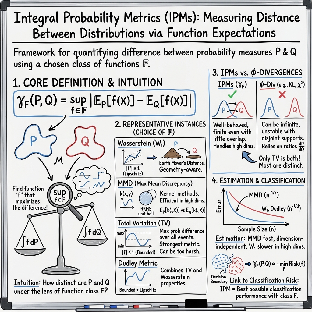
Integral Probability Metrics Overview
- Integral Probability Metrics (IPMs) are distance measures defined by the supremum difference in expectations over chosen function classes, comparing probability distributions.
- They include metrics like Wasserstein, MMD, Dudley, and Total Variation, each designed for specific regularity and computation needs.
- IPMs underpin practical applications in machine learning and statistics by linking classifier risk with distributional discrepancies and enabling robust empirical estimation.
Integral Probability Metrics (IPMs) are a broad class of probability distances defined by taking the supremum of the difference in expectations of a function over two probability measures, where the function class is specified to capture certain regularity, geometry, or statistical properties. IPMs encompass distance measures such as the Wasserstein distance, Dudley metric, Total Variation, Maximum Mean Discrepancy, and others, and have become central to modern probability theory, machine learning, and statistics for tasks involving comparison, estimation, and learning with probability distributions.
1. Definition and Representative Instances
An Integral Probability Metric between probability measures and on a measurable space is given by
where is a class of real-valued, bounded, measurable functions on .
Examples of IPMs include:
- Wasserstein Distance ():
- , functions with Lipschitz constant at most 1.
- Dual form: .
- Dudley Metric ():
- , where .
- Maximum Mean Discrepancy (MMD):
- is the unit ball in a Reproducing Kernel Hilbert Space (RKHS).
- .
- Total Variation Distance (TV):
- .
- .
- Kolmogorov Distance:
- is indicator functions of half-infinite intervals on .
This framework includes many classical distances as special cases and can be tuned for the application by selecting appropriately.
2. Comparison with φ-Divergences and Theoretical Distinctions
The paper establishes that except for total variation, IPMs and φ-divergences (divergences defined by a convex function ) are fundamentally distinct. A φ-divergence has the form
for convex . Only the total variation distance is both an IPM and a non-trivial φ-divergence; all other principal φ-divergences (KL, χ², etc.) do not belong to the IPM family. This has important consequences:
- Properties of φ-divergences (such as those relying on absolute continuity) do not carry over to generic IPMs.
- In high-dimensional or low-overlap settings, φ-divergences may become infinite or poorly behaved, whereas IPMs (e.g., Wasserstein) remain defined and well-behaved.
3. Empirical Estimation and Computational Aspects
Given empirical measures from finite i.i.d. samples,
Estimation strategies depend on the chosen :
- Wasserstein/Dudley: Reduction to a linear program with constraints reflecting Lipschitz or bounded Lipschitz conditions.
- MMD: Closed-form, unbiased estimator involving only kernel evaluations, scalable to high dimensions.
- Total Variation: Direct empirical version is not always strongly consistent.
Consistency and Convergence:
- For MMD: Parametric convergence rate , dimension-independent.
- For Wasserstein and Dudley: Dimension-dependent rate .
- Empirical estimators can be computed efficiently for all sample sizes and tend to outperform φ-divergence estimators, which struggle in high dimensions and with disjoint supports.
4. Connection to Binary Classification
The IPM between two class-conditional distributions is directly related to the minimal risk of a binary classifier from a function class : where is a specifically chosen loss function depending on class priors. Thus:
- The IPM reflects the best achievable (negative) classification risk for a given class of functions.
- For different , this yields:
- Wasserstein: Optimal risk for Lipschitz classifiers.
- MMD: For kernel classifiers.
- TV: For all bounded classifiers.
- The "margin" or smoothness of the optimal classifier is linked to the IPM—lower IPM implies higher complexity (less smooth) classifiers are needed to distinguish the classes.
5. Practical Implications and Applications
Statistical advantages:
- Robustness: IPMs are sensitive to all differences between distributions, not just those detectable by φ-divergences.
- Computational feasibility: Linear programs or closed-form solutions make many IPMs readily usable in practice.
- Dimension-independence: MMD and similar kernelized IPMs are attractive in very high-dimensional contexts.
Applications:
- Hypothesis testing, two-sample tests, goodness-of-fit.
- GANs and generative models as objectives to measure fit between real and generated distributions.
- Image processing, neuroscience, and any field where model-data comparison is central.
- Binary classification, with risk-minimization directly linked to measurable probabilistic distance between classes.
Summary Table of Major IPMs
| Metric | Function Class () | Key Properties |
|---|---|---|
| Wasserstein () | 1-Lipschitz | Weak topology, geometry |
| Dudley | BL-norm bounded () | Topology-refined |
| MMD | Unit ball in RKHS | Efficient, kernel-two-sample |
| Total Variation | Strongest, not always comput. | |
| Kolmogorov | Indicator functions | 1D; empirical CDF–based |
In conclusion, IPMs constitute a unified, effective, and tractable framework for quantifying distance between probability measures. They provide statistical, computational, and interpretive advantages over classical φ-divergences, and their deep connection to binary classification risk grounds them in decision-theoretic perspectives. For practical problems involving high dimensional data, small sample regimes, or low class overlap, IPMs—particularly Wasserstein, MMD, and suitable custom function classes—are often preferred for both empirical and theoretical analyses.
