Covariate-dependent Nonparametric -modeling for regression via infinite Mixture-of-Expertizing class
Abstract: Empirical Bayes -modeling captures unit-level heterogeneity by estimating a latent prior distribution from observed data. In the existing formulations, however, the prior is shared by all units. In this paper, we develop a covariate-dependent g-modeling framework for regression in which the entire prior distribution of the regression coefficients is allowed to depend on covariates. We formulate the estimation of the prior as nonparametric maximum likelihood estimation (NPMLE) of the covariate-dependent prior, and show that the unrestricted problem is ill-posed. To resolve this, we introduce the infinite Mixture-of-Expertizing class of conditional priors, under which the NPMLE is precisely a softmax-gated Mixture of Experts (MoE) whose number of experts is not fixed in advance but is determined by the data. Building on a first-order optimality condition, we propose two exemplar-based estimation algorithms that select experts automatically, together with a post-hoc aggregation of experts for interpretation. On the theoretical side, we show that every conditional prior in the class is Lipschitz continuous in the covariates, and that aggregated softmax gates can approximate any continuous gate function. The effectiveness of the proposed NPMLE is shown through application to synthetic datasets and real datasets.
Paper Prompts
Sign up for free to create and run prompts on this paper.
Top Community Prompts
Explain it Like I'm 14
1. What is this paper about?
This paper introduces a new statistical method for situations where different people, places, or groups may follow different relationships between causes and outcomes.
For example:
- The effect of income on house prices may differ between cities.
- A medical treatment may work differently for people of different ages or backgrounds.
- The connection between a person’s characteristics and their health may vary across regions.
The researchers want to estimate these changing relationships from data. Their main idea is to allow the distribution of regression effects to depend on additional information, such as location or demographic characteristics.
They call their approach covariate-dependent g-modeling. It combines ideas from:
- Empirical Bayes, a method for learning hidden patterns from data;
- Nonparametric maximum likelihood estimation, which estimates a distribution without forcing it to have a particular shape; and
- Mixture of Experts, a model that combines several smaller prediction models.
2. What questions are the researchers asking?
The paper focuses on several main questions:
- How can we model differences between units? A “unit” might be a person, house, hospital, or geographic area. The researchers want each unit to have its own hidden regression coefficients rather than assuming that everyone follows exactly the same relationship.
- How can these hidden differences depend on covariates? The method should allow the distribution of effects to change depending on information such as location, age, or income.
- How can this distribution be estimated without assuming it is normal or follows another simple shape? Instead of choosing one fixed type of distribution, the researchers let the data reveal its shape.
- How can the method automatically decide how many different groups or “experts” are needed? Many mixture models require the researcher to choose the number of groups in advance. This paper proposes methods that can remove unnecessary groups automatically.
- Does the new method work in theory and in real examples?
3. How does the method work?
The basic regression idea
In an ordinary regression model, we might write:
House price = effect of income + effect of age of house + random error.
This assumes the effects are the same for every house.
The paper uses a more flexible idea. Each unit has its own hidden coefficient vector, written as . These coefficients describe how strongly different variables affect the result for that unit.
For example, one city might have a strong relationship between income and house prices, while another city might have a weaker relationship.
The researchers do not observe directly. They only observe the explanatory information and the outcome. They therefore try to infer the hidden coefficients from the data.
Two types of information: and
The method uses two sets of variables:
- describes the variables used directly to predict the outcome. For housing, these could include income, house age, and number of rooms.
- describes information that may explain why the regression relationships differ. For example, could contain latitude and longitude.
This means that two houses with similar characteristics may still have different effects because they are in different locations.
Learning a hidden distribution
Instead of estimating only one coefficient for each unit, the method estimates a distribution of possible coefficients.
This distribution is called a prior distribution. It represents the different kinds of relationships that may exist across units.
The important new feature is that this distribution can change with :
In simple language, this means:
The likely regression effects can be different in different places or for different types of people.
The method is called nonparametric because it does not assume that this distribution must be, for example, a bell-shaped normal distribution.
Why the straightforward approach fails
A simple approach would estimate a completely separate distribution for every observed value of .
However, if every unit has a different value of , the method could simply create a special answer for each individual observation. It might explain every data point perfectly, but it would not learn a useful general pattern.
This is called an ill-posed problem. It is similar to memorizing every answer on a test instead of learning the subject.
The Mixture-of-Experts solution
To prevent this problem, the researchers use a Mixture-of-Experts model.
Imagine several specialists, or “experts,” giving predictions:
- Expert 1 may represent areas where income has a strong effect.
- Expert 2 may represent areas where house age is especially important.
- Expert 3 may represent another pattern.
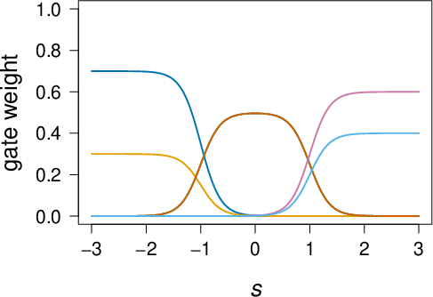
A gate decides how much attention to give each expert. The gate uses , such as geographic location, to calculate the weights.
For example, near one city the model might use:
- 70% Expert 1,
- 20% Expert 2,
- 10% Expert 3.
In another city, the weights may be different.
The paper uses a softmax gate, which is a mathematical way to turn several scores into positive percentages that add up to 100%.
The model therefore has:
- Experts: different regression relationships;
- Gates: rules that decide which experts matter in each situation; and
- A changing mixture: the experts’ importance changes according to the covariates.
How the number of experts is chosen
The researchers do not decide the final number of experts beforehand.
They begin with many possible candidate experts. During optimization, experts that are not useful receive a weight of zero and are removed. This lets the data select the effective number of experts.
They propose two related algorithms:
- Free-EXMoE: allows the regression coefficients of the experts to change during fitting;
- Grid-EXMoE: uses a prepared collection of candidate experts and mainly estimates their weights.
Both methods begin by creating exemplars. An exemplar is an initial guess for a possible expert. The researchers create these guesses by fitting small regression models to small, often nearby groups of observations.
Finally, they offer a method for combining similar experts so that the result is easier to understand.
4. What did the researchers find?
Theoretical findings
The paper proves several important mathematical facts.
The method avoids the worst form of overfitting
The unrestricted problem can produce meaningless solutions that memorize individual observations. Restricting the model to the proposed infinite Mixture-of-Expertizing class prevents this direct degeneracy.
A finite number of experts is enough
Although the model is defined using an “infinite” class of possible mixtures, the best estimated solution can be represented using a finite number of support points. The paper shows that the number is at most $2n$, where is the number of observations.
In practice, the algorithms usually select fewer useful experts.
The estimated prior changes smoothly
The researchers show that, under their conditions, the estimated distribution of regression coefficients changes in a controlled way as the covariates change. In mathematical language, it is Lipschitz continuous.
This means that small changes in location or another covariate cannot cause completely wild jumps in the estimated relationships.
The gates are flexible
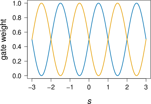
The paper also shows that combinations of softmax gates can approximate any smoothly changing set of expert weights.
In everyday terms:
If the true importance of different experts changes smoothly across space or across groups, the proposed model can represent that change as closely as needed.
Results from examples and applications
The authors test the method using simulated data and real datasets.
California housing data
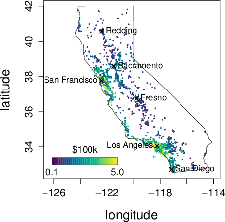
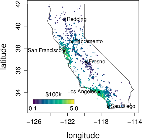
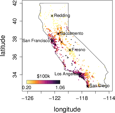
For the California housing data, the outcome is the median house value of a census area. Geographic coordinates are used as the covariates that control the gates.
The estimated distribution of regression coefficients changes as the model moves through different parts of California. For example, the relationship between house value and variables such as median income or house age differs across major cities.
This shows why a single shared distribution of regression effects would be too restrictive.
NHANES depression data
The paper also applies the method to depression scores from the National Health and Nutrition Examination Survey. This allows the researchers to study how regression relationships differ across people with different characteristics.
Simulated data
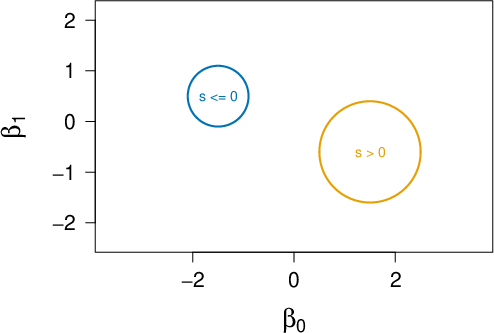
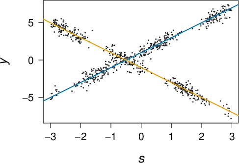
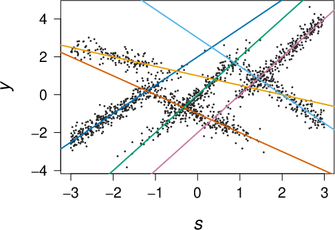
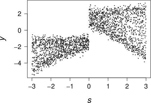
In simulations, the method is tested on data where the researchers know the underlying pattern. These experiments are used to check whether the method can recover changing groups of regression effects and select useful experts.
Overall, the examples suggest that the proposed method can detect structured differences that ordinary models with one shared prior may miss.
5. Why is this research important?
Many statistical models assume that one relationship applies to everyone. That assumption is often unrealistic.
The method in this paper is useful because it separates variation into two parts:
- Variation explained by observed information, such as location, age, or income; and
- Remaining individual variation among units that look similar.
This can provide a more detailed picture than simply reporting one average effect.
Possible uses include:
- Finding how medical treatments work differently for different populations;
- Understanding how housing markets vary from place to place;
- Studying regional differences in health or education;
- Improving predictions by choosing the most relevant expert for each case; and
- Helping researchers interpret hidden groups without deciding their number in advance.
The main limitation is that the method is mathematically and computationally more complicated than ordinary regression. It may also depend on choices such as the possible range of coefficients, the starting exemplars, and the regularization settings.
Still, the paper’s main contribution is a flexible way to model changing relationships:
Instead of assuming that all units share the same hidden pattern, the method allows the pattern itself to change with the units’ characteristics, while still keeping the model organized and interpretable.
Knowledge Gaps
Knowledge gaps, limitations, and open questions
- Identifiability of the conditional prior is not established. The paper does not determine when distinct mixing measures induce the same conditional prior or the same observed-data likelihood, particularly under finite samples and limited variation in and .
- The statistical consistency of the iMoE-NPMLE remains unresolved. No results are provided for consistency of or as , including weak convergence, convergence of conditional moments, or convergence of the induced marginal density.
- Rates of estimation are unknown. The paper does not derive finite-sample error bounds or minimax rates for estimating the covariate-dependent prior, its gates, or the regression-coefficient distribution.
- The effect of estimating the prior on unit-level posterior inference is not quantified. Although the framework is motivated by empirical Bayes inference, uncertainty in is not propagated to posterior estimates, credible intervals, shrinkage estimates, or decision rules for individual units.
- The restriction to the iMoE class may exclude important conditional priors. The model requires the conditional distribution to arise from an exponential tilting of a joint measure on , with shared support points in across . The paper does not characterize which covariate-dependent priors cannot be represented or approximated under this restriction.
- Approximation guarantees are incomplete. The universal approximation result concerns continuously varying gate functions after aggregation, but does not establish approximation of arbitrary conditional prior measures in a metric such as Wasserstein, total variation, or weak distance.
- The approximation theorem does not address the regression observation model. It remains unclear how accurately the proposed class approximates conditional marginal response densities, posterior distributions, or predictive quantities when the support points of the prior are also unknown.
- The imposed compact bounds and are not theoretically or practically justified. The paper does not explain how these sets should be selected, how sensitive estimates are to their boundaries, or what happens when the true coefficients or gate parameters lie outside them.
- The ridge-penalized implementation is not linked formally to the constrained iMoE-NPMLE. The theoretical estimator uses as a compact constraint, whereas Free-EXMoE replaces this with a penalty on . The relationship between the penalized solution and the original NPMLE is not established.
- The role and estimation of the dispersion parameter are left unspecified. Most procedures appear to treat as known, and the paper does not analyze joint estimation, misspecification, or the impact of dispersion uncertainty.
- The first-order optimality condition is only shown to be necessary. Because of the normalizing constants , the paper does not establish sufficiency, so a fitted measure satisfying the diagnostic may still be substantially suboptimal.
- Global optimization is not guaranteed. Free-EXMoE and Grid-EXMoE are explicitly designed to find local maximizers, but no conditions are given under which the algorithms reach the global NPMLE or approximate it reliably.
- The behavior of the algorithms under poor initialization is unknown. The empirical effect of the number of restarts, exemplar quality, initialization of , and initialization of support points is not theoretically characterized.
- There is no convergence analysis for the block-coordinate optimization. The paper does not prove convergence of the combined simplex, gate-parameter, and regression-coefficient updates, especially when inner optimization is approximate and active supports change.
- Automatic expert-number selection is not theoretically validated. Although zero weights remove candidate experts, the paper does not establish that the selected number of active experts is consistent, stable, or related to the effective complexity of the true prior.
- The bound of $2n$ support points is not shown to be practically sharp. It is unclear how often the NPMLE reaches this bound, how the required number of experts scales with covariate dimension, or whether smaller representations can be guaranteed.
- The post-hoc aggregation procedure lacks formal guarantees. The paper does not specify conditions under which merging experts preserves likelihood, predictive accuracy, prior moments, or approximation error.
- The choice of similarity criterion for expert aggregation is not fully justified. The consequences of clustering experts by proximity of while aggregating their gates are not analyzed when experts have similar coefficients but very different gate parameters, or vice versa.
- The sparse-representation result for does not translate into a comparable computational guarantee for . Since gate parameters must use all observations, the computational and statistical cost of estimating high-dimensional remains unresolved.
- High-dimensional covariate behavior is largely unexplored. The paper notes that gate grids grow exponentially with , but does not provide dimension-adaptive methods, sparsity guarantees, or theoretical results for large .
- The framework does not address regularization or variable selection for and . There is no treatment of sparse regression coefficients, sparse gate parameters, interactions, nonlinear covariate effects, or principled selection between variables entering the likelihood and variables entering the prior.
- The assumed linear softmax gate may be restrictive. The paper does not investigate nonlinear gates, interactions, basis expansions, neural gates, or other flexible parameterizations, nor their effect on identifiability and estimation.
- Covariate extrapolation is not studied. The behavior of outside the observed covariate region is not characterized, even though softmax gates can change substantially under extrapolation.
- The method’s sensitivity to the geometry and scaling of is unresolved. Because the gate depends on , estimates may be highly affected by covariate scaling, distance metrics used for anchored exemplars, and coordinate systems such as geographic latitude and longitude.
- The treatment of spatial dependence is incomplete. Geographic coordinates are used as covariates, but the model assumes conditional independence across units and does not account for spatial autocorrelation, spatially structured residuals, or irregular sampling.
- The interpretation of as explaining heterogeneity is not causally justified. The framework is associational; it does not distinguish genuine effect modification from confounding, selection effects, or measurement artifacts in the covariates.
- The model assumes independent latent coefficients conditional on covariates. Possible dependence among units, hierarchical clustering, temporal dependence, and shared latent shocks are not considered.
- The consequences of misspecifying the exponential-family likelihood are not analyzed. Robustness to overdispersion, zero inflation, heavy tails, link-function misspecification, and responses outside the assumed family remains unknown.
- The method is not evaluated for missing, noisy, or measured-with-error covariates. The framework assumes observed and are available without error, leaving practical data-quality issues unaddressed.
- The simulations and applications do not establish broad empirical robustness. The reported evaluations do not systematically vary sample size, dimensions and , overlap among gates, signal-to-noise ratio, support separation, covariate imbalance, or degree of prior misspecification.
- Comparisons with relevant alternative models are limited. The paper does not comprehensively compare against hierarchical random-coefficient models, varying-coefficient models, Bayesian nonparametric conditional priors, standard MoE models with fixed expert counts, or covariate-dependent parametric empirical Bayes methods.
- Uncertainty quantification is absent. No standard errors, confidence regions, bootstrap procedures, posterior uncertainty measures, or uncertainty bands for estimated gates and conditional prior summaries are developed.
- The finite-sample validity of the first-order diagnostic is unknown. The paper does not quantify how close the directional derivative must be to zero in practice or how the diagnostic should be calibrated to distinguish optimization failure from sampling variability.
- The unrestricted ill-posedness argument does not fully characterize alternative regularization strategies. The paper establishes degeneracy for the naive estimator but does not compare the iMoE restriction with smoothing penalties, kernel methods, Gaussian-process priors, or other ways to regularize .
- The interpretation of “irreducible” heterogeneity is not identified. Variation remaining in at similar covariate values may reflect omitted covariates, measurement error, model misspecification, or genuine individual-level randomness; the framework does not separate these sources.
- The impact of duplicate or nearly duplicate support points is not resolved. Softmax representations can be nonunique when experts have identical or similar values, and the paper does not provide a canonical representation or stability analysis for such cases.
- Theoretical results rely on continuity and positivity assumptions that may fail in common models. Boundary cases for Bernoulli, Poisson, gamma, or other exponential-family models, as well as responses with zero likelihood under some parameter values, are not treated.
- The method’s computational scalability is not demonstrated for genuinely large datasets. The paper does not provide complexity guarantees, memory analyses, distributed implementations, or approximation methods for large , large , or large numbers of candidate exemplars.
- The effects of local exemplar selection are not formally understood. The use of nearest neighbors in presumes that nearby units have similar latent coefficient distributions, but no conditions quantify when this assumption improves estimation or when it introduces bias.
- No principled method is given for selecting exemplar hyperparameters. The pool size , subset size , number of exemplars , grid resolution, penalty , and restart count are treated as tuning inputs without a general selection procedure.
- Predictive performance and decision-theoretic benefits are not fully characterized. The paper demonstrates estimation of covariate-dependent priors, but does not establish whether this improves out-of-sample prediction, individualized decisions, ranking, or compound-decision risk relative to simpler baselines.
Practical Applications
Immediate Applications
- Geographically varying housing-price models — real estate and urban analytics.
- neighborhood-specific price prediction;
- identification of housing submarkets;
- maps showing how the effect of a feature changes spatially;
- appraisal and valuation tools that provide both predictions and interpretable local coefficient distributions.
- This is directly motivated by the California housing analysis. It is deployable now for datasets containing geographic coordinates and sufficiently informative housing covariates. Feasibility depends on selecting bounded parameter regions and , having adequate observations across geographic areas, and avoiding excessive extrapolation beyond the observed spatial domain.
- Heterogeneous treatment-effect and risk-effect estimation — healthcare and epidemiology.
- subgroup-specific treatment-effect distributions;
- patient-level posterior coefficient estimates;
- identification of populations with unusually strong or weak treatment responses;
- risk models that separate covariate-explained heterogeneity from residual individual heterogeneity.
- This is an immediate methodological application, but clinical deployment requires validation, careful handling of confounding, and a defensible causal interpretation. The paper estimates conditional associations unless treatment assignment and confounding are explicitly addressed.
- Covariate-aware empirical Bayes shrinkage — statistics and quantitative decision support.
- small-area estimation;
- disease-risk estimation for individuals or institutions;
- insurance or credit-risk modeling;
- educational outcome prediction;
- personalized ranking or recommendation systems.
- The key dependency is that the new unit’s value should lie within, or close to, the training covariate region. Posterior quality also depends on correct specification of the exponential-family response and dispersion parameter.
- Interpretable mixture-of-experts modeling — software and machine learning.
Free-EXMoE and Grid-EXMoE can be implemented as an alternative to conventional MoE training when the number of experts is unknown. A practical software workflow would:
- generate local GLM exemplars from anchored subsets;
- initialize candidate experts;
- optimize gates, expert coefficients, and mixture weights;
- set redundant weights to zero through the simplex update;
- aggregate similar experts for interpretation;
- check the first-order optimality diagnostic. This provides automatic expert selection without repeatedly fitting models for many predetermined values of . Immediate use is most plausible for moderate-sized tabular datasets and standard Gaussian, Bernoulli, Poisson, or gamma responses. Non-convex optimization, initialization sensitivity, regularization choices, and computational cost remain important limitations.
Spatially varying coefficient visualization — public policy and regional planning.
- mapping the distribution of the income effect on housing values;
- locating regions where an environmental exposure has a different estimated health association;
- comparing regional responses to employment, education, or infrastructure policies.
- The method is immediately usable as an exploratory and diagnostic tool. Its policy interpretation depends on whether the covariates are predictive or causally interpretable, and on the stability of estimates in sparsely sampled regions.
- Subgroup discovery for education and social science.
- identifying school environments where teaching interventions have different associations with achievement;
- estimating heterogeneous relationships between family characteristics and educational outcomes;
- constructing subgroup-specific early-warning models.
- This can be deployed for exploratory analysis and targeted resource allocation. Dependencies include sufficient sample size within relevant regions of , protection against discriminatory use of sensitive attributes, and external validation before decisions are automated.
- NHANES-style population health stratification.
- prioritize screening or outreach;
- compare heterogeneous risk patterns across population groups;
- identify variables whose associations differ across age, income, or sex strata.
- Immediate deployment should be limited to descriptive and predictive analyses unless survey weights, complex sampling, missingness, and causal assumptions are incorporated appropriately.
- Model diagnostics and expert reduction.
- candidate experts that do not satisfy the estimated optimality conditions;
- experts with negligible gate mass;
- multiple experts with nearly identical regression coefficients;
- regions of covariate space where the fitted gates change sharply.
- This can reduce model size and improve communication to domain experts. Its reliability depends on numerical convergence and on the quality of the selected tolerances and aggregation thresholds.
Long-Term Applications
- Personalized treatment selection and precision medicine — healthcare.
- posterior treatment-effect distributions;
- uncertainty and confidence for each patient;
- similarity to previously observed patient subgroups;
- expected benefit under alternative interventions.
- This requires substantially more than predictive fitting: causal identification, longitudinal modeling, treatment-policy evaluation, prospective clinical validation, fairness assessment, and regulatory approval.
- Dynamic and longitudinal heterogeneous-effects models.
- personalized disease progression models;
- time-varying treatment response;
- patient-specific relapse or hospitalization risk;
- adaptive interventions.
- Dependencies include handling within-unit dependence, temporal drift, time-varying confounding, and computational scaling of exemplar generation and gate estimation.
- Large-scale adaptive mixture-of-experts systems — AI and software infrastructure.
- tabular-data MoE libraries with automatic expert-number selection;
- interpretable routing based on demographic, geographic, or operational context;
- hybrid neural-statistical models in which neural representations feed the gates while experts retain GLM structure;
- distributed training procedures that select and merge experts across data silos.
- Scaling to millions of observations or high-dimensional requires distributed optimization, approximate likelihood calculations, streaming exemplars, and safeguards against gate collapse or overly specialized experts.
- Fairness-aware and subgroup-robust decision systems.
- compare conditional priors across demographic groups;
- detect groups for which model errors or feature effects differ;
- impose fairness constraints on gates or expert predictions;
- quantify residual heterogeneity within groups.
- This requires careful decisions about which covariates may be used, protection against reconstructing sensitive attributes, fairness definitions appropriate to the application, and validation that expert aggregation does not conceal important subgroup differences.
- Policy simulation under regional heterogeneity.
- regional policy-impact distributions;
- uncertainty-aware budget allocation;
- identification of areas with distinct intervention responses;
- scenario analysis for housing, employment, education, or public health.
- This depends on causal model extensions, policy-invariant assumptions, representative data, treatment-effect transportability, and mechanisms for incorporating survey design and administrative-data bias.
- Robotics and autonomous systems with context-dependent dynamics.
- context-dependent motion or dynamics models;
- adaptive controller selection;
- fault detection through shifts in the inferred coefficient distribution;
- interpretable mixtures of operating modes.
- Practical deployment requires sequential data, state dependence, online updating, safety guarantees, and extensions beyond independent exponential-family responses.
- Energy demand, reliability, and grid operations.
- heterogeneous responses to temperature or pricing;
- region-specific renewable-generation behavior;
- distributions of equipment-failure or efficiency coefficients;
- adaptive demand-response policies.
- Dependencies include temporal and spatial dependence, nonstationary weather regimes, missing sensor data, extreme-event behavior, and integration with physical constraints and power-system simulators.
- Finance and insurance with context-dependent risk distributions.
- credit-risk models with subgroup-specific coefficient distributions;
- insurance pricing with heterogeneous claim-response relationships;
- stress testing under changing economic conditions;
- anomaly detection when a unit’s posterior is inconsistent with its contextual prior.
- Deployment requires strict controls for regulatory compliance, interpretability, discrimination, distribution shift, privacy, and the consequences of using sensitive covariates in gate functions.
- Continuous-gate and nonparametric prior modeling beyond softmax gates.
- smooth spatial coefficient fields;
- monotonic or shape-constrained gates;
- uncertainty bands for the entire prior ;
- Bayesian or conformal uncertainty quantification for predictions and expert assignments.
- Such extensions require stronger identifiability results, rates of convergence, principled regularization, uncertainty quantification, and methods for selecting the effective complexity of the gate.
- Scalable, theory-backed automated model selection.
- statistically justified expert-number selection;
- global or near-global optimization guarantees;
- confidence sets for support points and gates;
- stable results across random restarts;
- scalable approximation for very large , , or .
- These developments are necessary before the approach can serve as a general-purpose production modeling platform in high-stakes or high-volume applications.
Glossary
- Argmax: The set of parameter values that maximize a function. “”
- Canonical parameter: The natural parameter used to express an exponential-family distribution. “Here and are a canonical parameter and a dispersion parameter, respectively.”
- Carathéodory’s theorem: A convex-geometry result stating that a point in a finite-dimensional convex hull can be represented using a bounded number of points. “Thus, from the Carathéodory's theorem, the solution is represented as a convex combination of at most $2n$ points”
- Compound decision theory: A decision-theoretic framework that jointly considers decisions across multiple statistical units. “This setting, in which unit-level parameters are drawn from an unknown prior, is the classical setting of empirical Bayes (EB) and compound decision theory”
- Conditional marginal likelihood: The likelihood obtained by integrating latent parameters out of a model conditional on observed covariates. “where is the conditional marginal likelihood integrated over ”
- Conditional prior: A prior probability distribution whose parameters or entire distribution depend on observed covariates. “we develop a covariate-dependent -modeling framework in which the prior of the latent regression coefficients depends on covariates”
- Convex hull: The smallest convex set containing a given collection of points. “”
- Covariate-dependent heterogeneity: Variation among units that is systematically related to observed covariates. “Capturing such covariate-structured heterogeneity requires the prior to vary with the covariates.”
- Degenerate solution: A solution concentrated at a single parameter value, often producing an undesirable or ill-posed fit. “there are infinitely many degenerate trivial solutions”
- Directional derivative: The instantaneous rate of change of a function in a specified direction. “The directional derivative of the marginal log-likelihood with respect to along with point mass is given by”
- Dispersion parameter: A parameter controlling the variability of an exponential-family distribution beyond its mean structure. “ denotes an exponential family distribution with conditional mean and dispersion parameter .”
- Empirical Bayes: A Bayesian approach in which an unknown prior distribution is estimated from observed data. “The paradigm of estimating the prior from the observations is known as -modeling”
- Exemplar method: An estimation procedure that constructs candidate mixture components from solutions fitted to small subsets of observations. “For the unit-level Gaussian linear model, \cite{Jiang2025-am} recently provided a theoretical justification of NPMLE together with a practical estimation procedure called the exemplar method.”
- Exponential family: A broad class of probability distributions represented using a common exponential-form density. “These conditions are satisfied by the standard exponential families, such as the Gaussian, Bernoulli, Poisson, and gamma distributions”
- First-order optimality condition: A necessary condition involving derivatives that a differentiable objective satisfies at an optimum. “The following theorem states the first-order optimality condition with respect to .”
- Frank–Wolfe method: An iterative constrained optimization algorithm that updates a point toward a solution of a linearized objective over a feasible set. “Our default update rule is the pairwise Frank--Wolfe method”
- g-modeling: Estimation of a latent prior or mixing distribution from observed data. “The paradigm of estimating the prior from the observations is known as -modeling”
- Gate: A covariate-dependent weighting function that determines the contribution of each expert in a mixture-of-experts model. “the covariate-dependent weight functions are called gates and the component densities are experts.”
- Generalized linear model (GLM): A regression model in which a response distribution belongs to the exponential family and its mean is linked to a linear predictor. “We consider the unit-level generalized linear regression model (unit-level GLM) formulated as”
- Ill-posedness: A failure of a statistical optimization problem to have a stable, unique, or meaningful solution. “The direct extension of the NPMLE \eqref{def:NPMLE_regression} that maximizes over all conditional priors is ill-posed”
- Infinite Mixture-of-Expertizing (iMoE) class: A class of covariate-dependent priors formed by normalizing mixtures of softmax-weighted components, including non-finite mixing measures. “we employ the following infinite Mixture-of-Expertizing (iMoE) class of conditional probability measures.”
- Inverse link function: A function mapping a linear predictor to the mean of the response distribution. “ is a known inverse link function”
- Lipschitz continuity: A smoothness property in which function changes are bounded proportionally to changes in its input. “every conditional prior in the class is Lipschitz continuous in the covariates”
- Latent regression coefficient: An unobserved regression parameter associated with an individual unit. “where is a latent regression coefficient vector for unit ”
- Linear predictor: A linear combination of covariates and regression coefficients used to determine the response mean. “ is a linear predictor”
- Marginal likelihood: The likelihood obtained after integrating over unobserved or latent parameters. “the NPMLE is defined as”
- Mixture-of-Experts (MoE): A model that combines multiple component models using input-dependent mixing weights. “the conditional marginal density is precisely a Mixture-of-Experts (MoE) model”
- Mixing measure: A probability measure specifying the weights and parameters of a mixture distribution. “For a mixing probability measure ”
- Nonparametric maximum likelihood estimation (NPMLE): Maximum likelihood estimation over a broad class of probability distributions rather than a fixed finite-dimensional family. “We formulate the estimation of the prior as nonparametric maximum likelihood estimation (NPMLE)”
- Posterior inference: Inference about latent quantities using their distribution conditional on observed data. “The estimated prior enables unit-level posterior inference”
- Prior probability measure: A probability distribution assigned to latent parameters before observing the response data. “”
- Regularization: The addition of a penalty or constraint to stabilize estimation or prevent overly complex solutions. “with a regularization parameter .”
- Softmax gate: A normalized exponential function that converts component scores into covariate-dependent mixture weights. “The softmax gate is the vector-valued function”
- Support point: A parameter value receiving positive probability under a discrete probability measure. “where is some integer less than $2n$”
- Universal approximation theorem: A result establishing that a model class can approximate a broad class of target functions arbitrarily well. “the universal approximation theorem for the aggregated softmax gates.”
- Variance function: A function describing how the variance of an exponential-family distribution depends on its mean. “let denote the variance function of the exponential family.”
- Weighted GLM score equation: A likelihood-based estimating equation for a generalized linear model in which observations contribute unequally. “each support point solves a weighted GLM score equation.”

