On the Growth Factor of Random Matrices
Abstract: Gaussian elimination is the oldest and most popular method for solving a linear system. Its numerical stability for a given matrix is controlled by the growth factor, a measure of how large entries can become during elimination. In this work, we prove a number of new results regarding the growth factor of random matrices. First, we provide tight estimates for the growth factor of a matrix preconditioned by a Haar orthogonal matrix without pivoting and characterize the asymptotic distribution of the growth factor of Gaussian matrices without pivoting. Second, and most notably, we prove that the growth factor of an Gaussian matrix under partial pivoting is rarely much larger than , resolving an old conjecture of Nick Trefethen. The same techniques used to prove this conjecture also provide an improved smoothed analysis of the growth factor under partial pivoting.
Paper Prompts
Sign up for free to create and run prompts on this paper.
Top Community Prompts
Explain it Like I'm 14
1. What is this paper about?
This paper studies how numbers can grow during Gaussian elimination, a common method computers use to solve systems of equations.
When a computer uses Gaussian elimination, some numbers inside the matrix can become much larger than the original numbers. The paper studies this problem using random matrices, especially matrices whose entries are random numbers from a normal, or Gaussian, distribution.
The main question is:
How large do the numbers usually become when Gaussian elimination is used?
This matters because very large numbers can cause rounding mistakes in computers and make the calculation unstable.
2. Main research questions
The paper focuses on several related questions:
- What happens when Gaussian elimination is used without rearranging rows?
- Can randomly rotating a matrix before elimination prevent numbers from growing too much?
- How well does partial pivoting work? Partial pivoting means choosing the largest available number in a column as the next “pivot” and swapping rows if needed.
- What happens if a matrix is slightly disturbed by random noise? This is called smoothed analysis. It asks whether a small random change makes difficult examples less dangerous.
The most important question is about a long-standing conjecture by mathematician Lloyd Trefethen:
For a random Gaussian matrix, is the growth factor usually about when partial pivoting is used?
Here, is the size of the matrix.
3. How the researchers studied the problem
Gaussian elimination and the growth factor
Gaussian elimination changes a matrix step by step until it becomes easier to solve. It can also be described as factoring a matrix into two simpler matrices:
The matrix contains information about the elimination steps, while is an upper-triangular matrix containing the resulting values.
The paper measures the danger of the calculation using the growth factor:
In simple terms, this asks:
How much larger can the biggest number become during elimination compared with the biggest number we started with?
A small growth factor usually means the calculation is numerically stable. A large growth factor means rounding errors could become important.
Random matrices
The researchers mainly used Gaussian matrices. Each entry is chosen independently from a bell-shaped distribution centered at zero. This is similar to repeatedly rolling a special random-number generator.
They then:
- performed elimination with no pivoting;
- performed elimination with partial pivoting;
- studied matrices multiplied by random orthogonal matrices, which act like random rotations or reflections;
- added small Gaussian noise to fixed matrices;
- used probability estimates to show that bad outcomes are very unlikely.
Technical ideas in everyday language
The proofs use several advanced tools:
- Singular values: These describe how much a matrix stretches or shrinks different directions. Very small singular values can make elimination unstable.
- Schur complements: These are the smaller matrices that remain after some rows and columns have been eliminated.
- Probability bounds: These estimate how likely it is for a very large number to appear.
- High-probability results: A statement such as “with probability at least ” means that failure becomes extremely unlikely as the matrix gets larger.
- Smoothed analysis: Instead of studying a matrix exactly as it is, the researchers add a small random disturbance and study the result. This is like checking whether a slightly shaken version of a difficult situation becomes easier to handle.
A major part of the proof tracks the singular values of the smaller matrices that appear during elimination. The researchers show that, although some directions can be troublesome, random effects usually prevent these troublesome directions from causing very large entries.
4. Main findings
A. Random orthogonal preconditioning without pivoting
The paper first studies what happens if a fixed matrix is multiplied by a random orthogonal matrix before elimination, but no pivoting is used.
The researchers prove that the growth factor is usually no larger than roughly
apart from a small probability of failure.
A random orthogonal matrix is like randomly rotating the coordinate system. This can help, but the result shows that it is not as effective as partial pivoting for Gaussian matrices.
B. Gaussian matrices without pivoting
For an Gaussian matrix, the paper proves that the growth factor without pivoting is typically of size
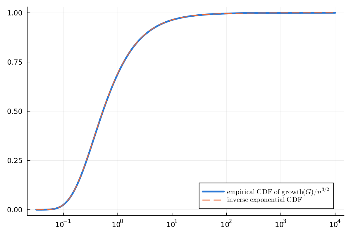
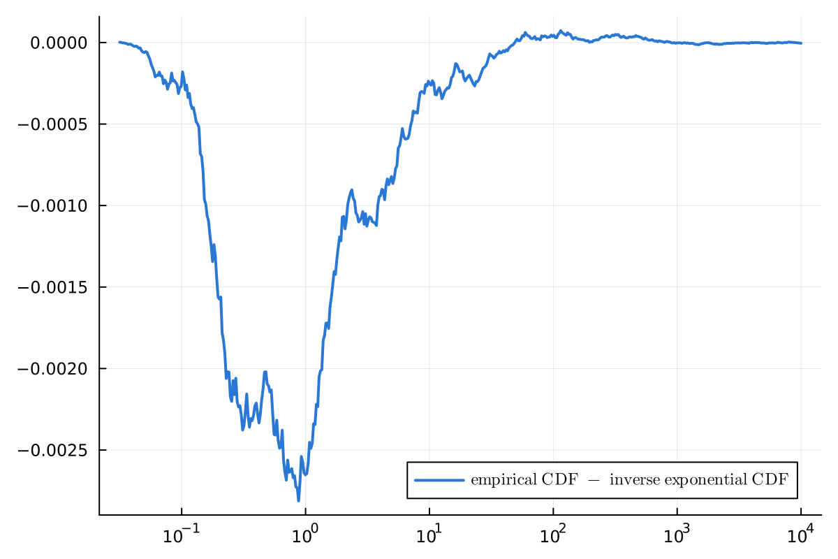
More precisely, after dividing the growth factor by , its probability distribution approaches an inverse exponential distribution.
This means that the growth factor is usually around the scale, but there is still a noticeable chance of unusually large values.
So, without pivoting, random matrices can experience much more growth than one might hope.
C. Gaussian matrices with partial pivoting
This is the central result.
The paper proves that for a Gaussian matrix, partial pivoting gives
with probability at least
for any fixed positive and sufficiently large .
The extra factor grows more slowly than any fixed power of . Therefore, the result is often summarized as
with overwhelming probability.
In simpler language:
For a large random matrix, partial pivoting usually keeps the growth factor close to , except for a very tiny chance of something much worse happening.
This proves Trefethen’s old conjecture.
The paper also shows that the exponent $1/2$ is essentially the best possible. In other words, is not just an upper-bound artifact; the growth factor really is at least about this large in typical cases.
D. Small random changes improve difficult matrices
The paper also studies a matrix of the form
where is any fixed matrix, is Gaussian noise, and controls the size of the disturbance.
The researchers prove that partial pivoting usually has a much smaller growth factor than previous results guaranteed. Their bound is roughly
The exact formula is technical, but the main message is simple:
Adding even a small amount of random noise makes extremely bad behavior much less likely.
This improves an older bound that allowed growth as large as approximately . The new result is closer to a polynomial bound, although the authors believe an even better polynomial estimate may be possible.
5. Why the findings matter
Partial pivoting is widely used in real software, including Python, MATLAB, and Julia. Before this paper, people had strong experimental evidence that it worked well for random matrices, but there was no complete mathematical proof of the expected behavior.
This paper provides that proof.
The results are important because they explain why partial pivoting is so successful in practice:
- In the worst possible case, partial pivoting can allow extremely large growth.
- But for random matrices, such bad behavior is extraordinarily unlikely.
- Without pivoting, growth is usually much larger, around .
- Random rotations can help, but generally not as much as partial pivoting.
- Small random perturbations can make even difficult matrices safer to handle.
Conclusion
The paper gives a mathematical explanation for the reliability of a method used by computers every day.
Its main lesson is:
Although Gaussian elimination with partial pivoting can fail badly on specially designed matrices, it is very unlikely to do so on a random matrix. For a random matrix, the growth factor is usually close to .
This supports the continued use of partial pivoting as a practical balance between safety and speed. The work may also help scientists design faster numerical algorithms and better understand how randomness protects computations from unstable behavior.
Knowledge Gaps
Knowledge gaps, limitations, and open questions
- The theorem for Gaussian matrices under partial pivoting gives an upper bound of , but does not determine the sharp asymptotic scale beyond the exponent $1/2$ or establish a tight multiplicative bound.
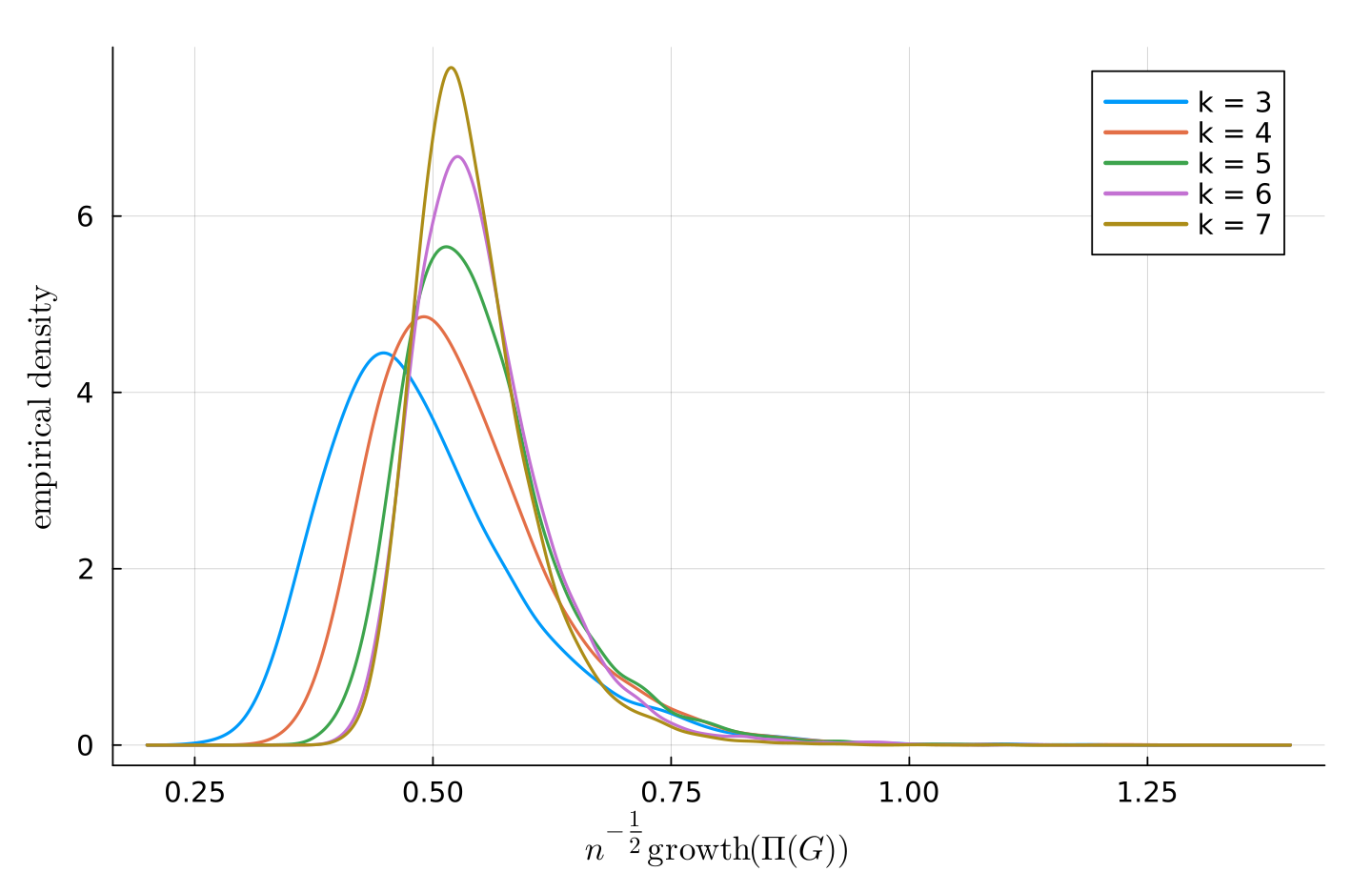
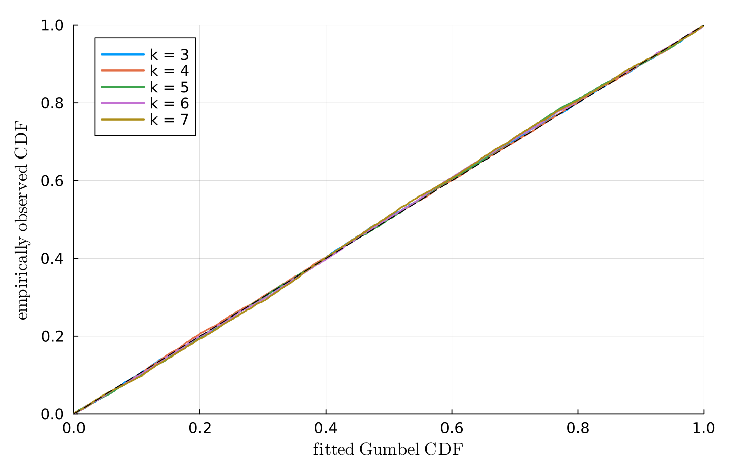
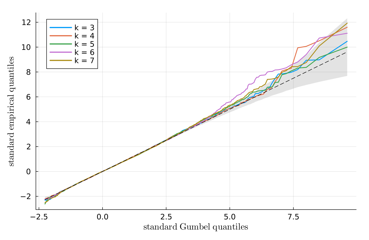
- The limiting behavior of remains unresolved: simulations suggest convergence to a constant or a suitably normalized Gumbel distribution, but neither possibility is proved.
- No limiting distribution, concentration inequality, or precise fluctuation scale is derived for the growth factor under partial pivoting.
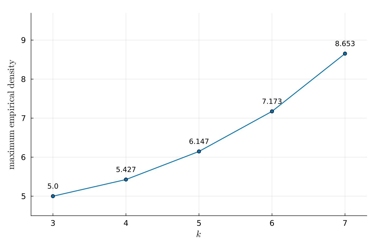
- The proof does not establish whether the empirical narrowing of continues asymptotically or is a finite-dimensional numerical artifact.
- The lower-bound argument for partial pivoting only establishes the logarithmic exponent $1/2$ and does not provide a sharp lower-order term or a matching high-probability lower bound for the growth factor.
- The analysis controls the truncated inverse quantities , but does not characterize their actual distribution, typical magnitude, or dependence on the pivot index .
- It remains unproved whether partial pivoting systematically improves , or other relevant inverse-norm statistics, relative to unpivoted Gaussian elimination; the paper explicitly identifies this as a difficult open problem.
- The results are restricted primarily to square real Gaussian matrices. Their extension to rectangular matrices, complex Gaussian matrices, or other rotationally invariant ensembles is not established.
- The robustness of the partial-pivoting result for non-Gaussian input distributions is unknown. In particular, universality under subgaussian, heavy-tailed, correlated, or discrete distributions is not proved.
- The paper does not determine whether finite-support discrete distributions exhibit the same -scale growth under partial pivoting as Gaussian matrices.
- The smoothed-analysis bound
is explicitly believed to be non-optimal. The conjectured polynomial dependence on and remains unproved.
- The optimal dependence of the smoothed growth factor on the perturbation size is unresolved, including whether polynomially small perturbations always yield polynomial growth with high probability.
- The smoothed-analysis result assumes and Gaussian perturbations; its dependence on other norms, perturbation distributions, matrix structures, and deterministic conditioning parameters is not investigated.
- No matching lower bounds are provided for the smoothed-analysis estimate, so it is unclear which parts of the dependence on and are intrinsic and which are artifacts of the proof.
- The theorem for Haar orthogonal preconditioning gives an tail bound, but does not determine the sharp tail behavior or limiting distribution of the growth factor for a fixed matrix .
- The claimed tightness of the exponent for non-adaptive orthogonal preconditioners is demonstrated through Gaussian matrices, but the optimal constants, tail exponents, and dependence on the deterministic matrix remain unknown.
- It is not established whether alternative randomized preconditioners, such as structured orthogonal, butterfly, subsampled randomized Fourier, or sparse transforms, can achieve growth closer to the partial-pivoting scale while retaining low computational cost.
- The comparison between orthogonal preconditioning and partial pivoting is made for Gaussian matrices, but no general comparison is proved for deterministic or structured input matrices.
- The paper analyzes exact-arithmetic growth factors and only discusses floating-point effects through references to prior work. A direct finite-precision version of the main probabilistic theorems, including pivot-selection perturbations and accumulation of roundoff error, is not developed.
- The effect of different tie-breaking rules, although negligible for continuous Gaussian inputs, is not studied for discrete or degenerate distributions where pivot ties can occur with positive probability.
- The results concern the maximum-entry growth factor, but do not directly quantify backward error, forward error, solution accuracy, or practical failure probabilities for linear systems solved using the analyzed random matrices.
- The dependence between pivot choices across elimination stages is handled indirectly through conditioning, but the resulting stochastic process of pivot locations is not characterized.
- The analysis does not explain the mechanism behind the apparent empirical Gumbel behavior or identify the effective number and dependence structure of the random variables whose maximum might determine the growth factor.
- The paper does not provide non-asymptotic distributional approximations or finite- error bounds for the inverse-exponential limit obtained for unpivoted Gaussian elimination.
- For unpivoted Gaussian elimination, the limiting inverse-exponential law is established for the growth factor but not for related quantities such as individual pivots, the largest Schur-complement entry, or the joint process across elimination stages.
- The effect of column pivoting, complete pivoting, rook pivoting, threshold pivoting, or hybrid pivoting rules on the sharp random-matrix growth scale remains unresolved.
- The techniques are not shown to apply to structured random matrices, including random orthogonal, Haar-unitary, Toeplitz, circulant, sparse, or covariance-type matrices.
- The paper does not investigate how matrix scaling, equilibration, sparsity, or low-rank structure alters the probabilistic growth-factor estimates.
- The technical singular-value bounds used in the proof are not shown to be optimal; sharper control of extreme singular values could potentially improve both the partial-pivoting and smoothed-analysis bounds.
- The consequences of the results for iterative refinement, mixed-precision LU factorization, and adaptive precision selection are left unexplored.
Practical Applications
Immediate Applications
- Reliable default linear-system solving in scientific and engineering software (software, scientific computing) Existing LU solvers using Gaussian elimination with partial pivoting can continue to serve as a computationally inexpensive default for systems whose inputs are approximately Gaussian, randomized, or otherwise sufficiently generic. The paper proves that, for an Gaussian matrix, the growth factor is at most
except with probability smaller than . This supports practical use of partial pivoting in numerical libraries such as MATLAB, Julia, and NumPy-based workflows without routinely switching to more expensive complete pivoting.
- Potential tool: solver diagnostics that estimate the observed growth factor during LU factorization and warn only when it is unusually large.
- Dependencies: the guarantee is probabilistic and is strongest for Gaussian or Gaussian-like data; adversarial or highly structured matrices can still exhibit exponential growth.
- Precision and overflow budgeting for LU factorization (high-performance computing, embedded computing, hardware design) The results can inform the number of guard bits, accumulator width, and overflow margins required by LU implementations. Since forward error bounds depend on the growth factor, the typical -scale behavior for Gaussian inputs provides a principled basis for setting precision policies rather than designing solely for the worst-case bound.
- Potential workflow: choose precision based on matrix dimension, machine epsilon, conditioning estimates, and a probabilistic growth-factor budget.
- Dependencies: growth factor does not replace the condition number; an ill-conditioned matrix may remain inaccurate even when element growth is moderate. Floating-point effects and pivot-selection changes must also be monitored.
- Runtime monitoring and adaptive solver selection (software, cloud computing) LU implementations can record the maximum magnitude of intermediate Schur-complement entries and compare it with -scale thresholds. If growth is unexpectedly high, the system can switch to complete pivoting, QR factorization, higher precision, or iterative refinement.
- Potential product: an adaptive numerical linear algebra runtime with policies such as:
- begin with partial pivoting;
- measure intermediate growth;
- escalate precision or change algorithms when a threshold is exceeded.
Dependencies: thresholds must account for matrix scaling, the norm of the input, and the distinction between exact-arithmetic and floating-point growth.
- Assessment of randomized and simulation-generated workloads (machine learning, statistics, finance, engineering simulation) Many design matrices, covariance-related matrices, Monte Carlo systems, and randomized test matrices are approximately Gaussian or contain substantial random perturbations. The theorem provides a theoretical benchmark for expected LU behavior on such workloads and can guide stress testing of solver implementations.
- Potential use: generate matrix-size-dependent test thresholds and compare production workloads against Gaussian baselines.
- Dependencies: approximate Gaussianity must be validated; correlations, sparsity, heavy tails, and deterministic structure may invalidate direct transfer of the result.
- Smoothed-analysis justification for perturbed numerical problems (optimization, control, inverse problems, numerical PDEs) For a matrix with perturbed as , the paper gives a high-probability bound of the form
This supports adding small randomized perturbations before factorization when the original input may be structured or near a numerically unfavorable configuration.
- Potential workflow: apply controlled Gaussian dithering, factor using partial pivoting, and quantify the perturbation size in the final error budget.
- Dependencies: perturbation may alter the original problem; the bound assumes a spectral-norm constraint on and does not establish that the resulting exponent is optimal.
- Empirical solver benchmarking and algorithm comparison (academia, numerical software development) The inverse-exponential limiting law for the growth factor of Gaussian matrices without pivoting provides a reproducible benchmark for testing LU implementations, pivoting heuristics, and random matrix generators. Small dimensions appear to converge rapidly to the predicted distribution, making the result useful for practical experiments.
- Potential tool: benchmark suites comparing no pivoting, partial pivoting, orthogonal preconditioning, and complete pivoting using normalized growth factors.
- Dependencies: the limiting law applies asymptotically and specifically to Gaussian matrices without pivoting; it should not be interpreted as a universal model for application matrices.
- Guidance against using unpivoted LU as a generic replacement for partial pivoting (software, education, engineering practice) The paper shows that Gaussian matrices without pivoting have growth on the scale, substantially larger than the scale established for partial pivoting. This gives a direct practical argument for retaining partial pivoting even when avoiding row exchanges appears attractive.
- Implication: unpivoted LU may be suitable only when matrix structure provides an independent stability guarantee, such as certain positive-definite or diagonally dominant settings.
- Dependencies: the comparison concerns element growth, not total runtime or parallel communication cost.
- Policy and procurement standards for numerical infrastructure (research computing, public-sector computing, finance, engineering regulation) Organizations can require numerical software to expose pivot-growth diagnostics, support fallback factorization methods, and document behavior on randomized and perturbed inputs. The results provide a mathematically grounded rationale for treating partial pivoting as a reliable baseline rather than requiring the cost of complete pivoting for every problem.
- Dependencies: standards should combine growth monitoring with conditioning, residual checks, reproducibility requirements, and application-specific accuracy criteria.
Long-Term Applications
- Probabilistically certified LU solvers (scientific computing, safety-critical software)
The results could support solvers that provide probabilistic certificates such as: “for a Gaussian-like input of dimension , the probability that growth exceeds the configured threshold is below .” Such certificates could be integrated with residual-based verification and condition estimation.
- Required development: extend the theory from exactly Gaussian matrices to correlated, sparse, heavy-tailed, block-structured, and data-dependent distributions.
- Key assumption: the input distribution must be characterized well enough for the probability guarantee to be meaningful.
- Distribution-aware automatic pivoting policies (software, HPC, numerical optimization)
Future factorization libraries could select among no pivoting, partial pivoting, randomized orthogonal preconditioning, and complete pivoting based on an online estimate of matrix structure. The paper suggests that orthogonal preconditioning without pivoting has -scale growth, whereas partial pivoting has -scale growth for Gaussian inputs, favoring partial pivoting in that regime.
- Potential product: a matrix analyzer that estimates Gaussianity, tail behavior, sparsity, conditioning, and observed growth before choosing a factorization strategy.
- Dependencies: reliable distribution detection and low-overhead policy selection remain open engineering problems.
- Randomized preconditioning for structured or adversarial matrices (optimization, PDEs, control, inverse problems)
The smoothed-analysis result suggests that adding calibrated random noise can suppress catastrophic growth for arbitrary norm-bounded matrices. This may lead to robust preprocessing layers for linear solvers applied to structured systems.
- Required development: determine perturbation levels that balance stability improvement against solution bias, privacy concerns, sparsity loss, and problem feasibility.
- Dependencies: the current bound is quasi-polynomial in the perturbation dependence and may be too pessimistic for large-scale deployment.
- Improved smoothed-analysis bounds and near-polynomial guarantees (academia, theoretical computer science) The paper improves earlier bounds to a dependence of approximately
A likely long-term objective is proving the conjectured polynomial behavior in both and . Such a result could yield stronger practical guarantees for perturbed worst-case inputs.
- Potential impact: formal stability guarantees for randomized numerical algorithms and more rigorous complexity estimates for linear-system solvers.
- Dependency: further control of extreme singular values and pivot-dependent submatrices is required.
- Finite-precision and hardware co-design based on probabilistic growth models (computer architecture, accelerators, FPGA/GPU design) The growth-factor laws could be incorporated into hardware that dynamically allocates exponent range, detects overflow risk, or changes precision during factorization. Specialized accelerators could exploit the typical rather than worst-case behavior of randomized workloads.
- Required development: establish equivalent guarantees directly for floating-point growth, including rounding accumulation, finite exponent ranges, mixed precision, and parallel pivoting.
- Dependencies: exact-arithmetic probabilistic bounds alone are insufficient for safety-critical hardware guarantees.
- Numerically robust randomized workflows in machine learning and data science (machine learning, statistics) Randomized regularization, dithering, and perturbation are already common in data processing. The paper’s smoothed-analysis framework could eventually inform principled perturbation schemes for least-squares systems, feature transformations, and covariance computations that rely on LU-like elimination.
- Potential workflow: normalize the matrix, add a controlled perturbation, perform partial-pivoted factorization, and certify residual and growth behavior.
- Dependencies: perturbations must not materially change statistical estimands, fairness properties, interpretability, or downstream model behavior.
- Extensions to block, sparse, distributed, and communication-avoiding elimination (HPC, distributed computing, robotics, large-scale simulation) The proof techniques involving Schur complements, truncated inverse norms, singular-value control, and conditional Gaussian structure may inspire analogous analyses for block LU and distributed factorization algorithms.
- Potential tools: block-pivot growth monitors, randomized communication-avoiding preconditioners, and distributed stability certificates.
- Dependencies: block pivoting changes the growth mechanism; sparsity patterns, fill-in, communication order, and dependence between blocks require new analysis.
- Applications to randomized robotics, finance, and control pipelines (robotics, finance, aerospace, energy) Many estimation, trajectory optimization, Kalman filtering, portfolio, and power-system calculations repeatedly solve linear systems. A mature distribution-aware stability framework could help determine when low-cost partial-pivoted LU is adequate and when QR, SVD, or higher precision is necessary.
- Required development: validate the random-matrix assumptions for time-correlated, streaming, constrained, and highly structured matrices encountered in these domains.
- Dependency: domain-specific failure costs may require much stronger guarantees than high-probability asymptotics provide.
Glossary
- Asymptotic distribution: The limiting probability distribution approached by a sequence of random variables as the dimension grows. “characterize the asymptotic distribution of the growth factor of Gaussian matrices without pivoting”
- Beta distribution: A continuous probability distribution on the interval , commonly used to model proportions and random variables derived from squared coordinates of uniformly distributed sphere points. “”
- Block inversion formula: An identity for computing the inverse of a partitioned matrix from the inverses and Schur complements of its blocks. “Then, by the block inversion formula”
- Butterfly matrix: A structured matrix composed of sparse, recursively arranged transformations, often used to reduce the cost of applying a matrix or preconditioner. “Butterfly matrices have also been considered as a potential preconditioner to limit growth”
- Conditioning: Analyzing a random quantity given that specified information or an event is known. “Our argument involves revealing pivot choices or columns of iteratively and conditioning.”
- Convex set: A set containing the line segment between any two of its points; convexity enables particular geometric and probabilistic inequalities. “ be distributed as conditioned on lying in a convex set ”
- Concentration inequality: A probabilistic bound showing that a random quantity is unlikely to deviate substantially from its typical value. “The desired result follows from Gaussian concentration”
- Complete pivoting: A Gaussian-elimination strategy that selects the largest-magnitude entry in the remaining submatrix as the next pivot, allowing both row and column permutations. “Complete pivoting has a growth factor which is only quasi-polynomial”
- Cumulative distribution function (CDF): A function giving the probability that a random variable is less than or equal to a specified value. “we compare their distributions directly”
- Frobenius norm: The square root of the sum of the squared magnitudes of all matrix entries, equal to the Euclidean norm of the matrix viewed as a vector. “the squared Frobenius norm of the inverse”
- Gaussian concentration: Concentration of Gaussian random variables or functions of Gaussian variables around their expected values. “and so, by Gaussian concentration”
- Gaussian elimination: An algorithm that solves linear systems by transforming a matrix into triangular form through row operations. “Gaussian elimination is the oldest and most popular method for solving a linear system.”
- Gaussian matrix: A matrix whose entries are independent standard normal random variables. “A matrix is said to be Gaussian if its entries are independent standard normal random variables.”
- Gaussian perturbation: A random additive modification whose entries are sampled from a Gaussian distribution. “any matrix plus a small Gaussian perturbation”
- Gumbel distribution: An extreme-value distribution that commonly models maxima of many random variables. “the fluctuations of , properly shifted and normalized, seem to resemble Gumbel distributions.”
- Haar measure: The unique uniform probability measure on a compact group that is invariant under group multiplication. “”
- Haar orthogonal matrix: An orthogonal matrix sampled uniformly according to Haar measure on the orthogonal group. “a matrix preconditioned by a Haar orthogonal matrix”
- Heavy tail: A probability distribution whose tail probabilities decrease relatively slowly, making unusually large values more likely than under light-tailed distributions. “ has a heavy tail and an infinite mean.”
- High probability: An event whose probability approaches one, typically at a specified asymptotic rate. “bounded by with high probability”
- Inverse exponential distribution: A distribution obtained by taking the reciprocal of an exponential-type random variable, with a heavy upper tail. “”
- Leading principal minor: The determinant of a submatrix formed from the first rows and first columns of a matrix. “given an matrix with non-zero leading principal minors”
- Lipschitz function: A function whose output changes by at most a fixed constant times the distance between inputs. “Both and are -Lipschitz”
- Moore–Penrose pseudoinverse: A generalized matrix inverse defined for rectangular or singular matrices and characterized by the Penrose equations. “Let denote the Moore-Penrose pseudoinverse”
- Non-degenerate distribution: A probability distribution that is not concentrated at a single value or otherwise lacking meaningful variability. “entries sampled independently from a non-degenerate discrete distribution with finite support”
- Orthogonal invariance: The property that a distribution remains unchanged under multiplication by orthogonal matrices. “By the orthogonal invariance of ”
- Partial pivoting: A Gaussian-elimination strategy that swaps rows so the largest-magnitude entry in the current column is selected as the pivot. “Gaussian elimination with partial pivoting is the standard linear system solver”
- Permutation matrix: A matrix obtained by permuting the rows or columns of an identity matrix. “it is represented mathematically by left-multiplication by a single permutation matrix ”
- Preconditioner: A transformation applied to a system or matrix to improve numerical stability or computational performance. “Butterfly matrices have also been considered as a potential preconditioner to limit growth”
- Quasi-polynomial: Having complexity or magnitude bounded by an expression such as , intermediate between polynomial and exponential. “Complete pivoting has a growth factor which is only quasi-polynomial”
- Rank-one transformation: A matrix update or operation whose change has rank one. “the procedure performs a series of rank-one transformations”
- Schur complement: The matrix obtained after eliminating a block of variables from a block-partitioned matrix. “where is the Schur complement of with respect to the submatrix ”
- Singular value: The nonnegative square-root eigenvalues of , measuring the scaling of a matrix along orthogonal directions. “We denote the singular values of a matrix ”
- Slutsky’s theorem: A result stating that convergence in distribution is preserved under multiplication or addition with quantities converging in probability to constants. “by Slutsky's theorem”
- Smoothed analysis: Analysis of an algorithm’s performance after applying a small random perturbation to its input. “smoothed analysis, which considers the performance of an algorithm under small random perturbations to the input.”
- Spectral recursion: A recursive argument that tracks or bounds quantities associated with eigenvalues or singular values across successive matrix stages. “with a number of key refinements and differences in our spectral recursion”
- Sub-Gaussian: Having tails that decay at least as rapidly as Gaussian tails, often characterized through moment-generating-function bounds. “retains enough ``Gaussianity'' for our purposes”
- Submatrix: A matrix formed by selecting a subset of the rows and columns of another matrix. “the inverse of a submatrix of a Haar orthogonal matrix”
- Subspace: A subset of a vector space closed under vector addition and scalar multiplication. “the column space of and ”
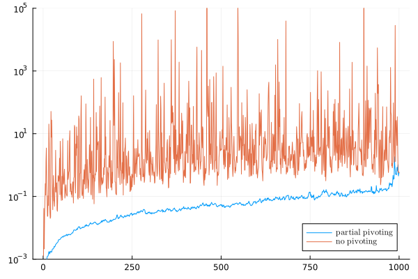
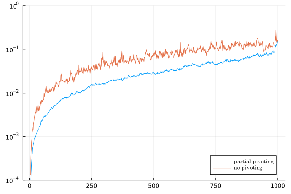
- Tail distribution: The probability that a random variable exceeds a specified threshold. “The empirical difference in tail distribution between no pivoting and partial pivoting”
- Truncated inverse: An inverse whose largest singular-value contributions have been removed from a norm or spectral sum. “the Frobenius norms of the truncated inverses”
- Union bound: The inequality that bounds the probability of a union of events by the sum of their individual probabilities. “where the second estimate follows from a union bound”
- QR factorization: A decomposition of a matrix into the product of an orthogonal matrix and an upper triangular matrix. “by and the QR factorization”
- Quasi-polynomial growth: Growth bounded by a quasi-polynomial rather than a polynomial or exponential function. “Complete pivoting has a growth factor which is only quasi-polynomial”
- With overwhelming probability: With probability tending to one faster than any fixed inverse polynomial in the dimension. “at most with overwhelming probability”

