Bounded gaps between primes
Abstract: Polymath8b proved that . In this paper we show how the Bombieri-Vinogradov theorem can be combined with newer equidistribution estimates for smooth moduli to obtain the improved bound .
Paper Prompts
Sign up for free to create and run prompts on this paper.
Top Community Prompts
Explain it Like I'm 14
1. What is this paper about?
This paper studies how close two consecutive prime numbers can be.
Prime numbers are numbers such as $2,3,5,7,11,$ and $13$ that can only be divided evenly by $1$ and themselves. Sometimes two primes are close together, like $11$ and $13$, which have a gap of $2$.
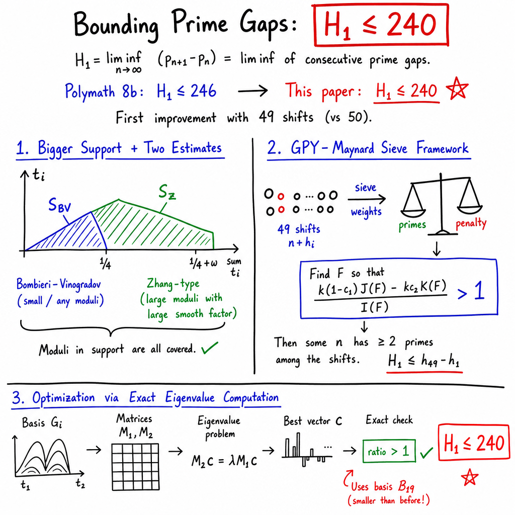
The paper improves an earlier result that showed there are infinitely many pairs of consecutive primes with a gap of at most 246. The new result proves that there are infinitely many such pairs with a gap of at most 240.
In symbols, the paper proves
This means that no matter how far we go along the number line, we will keep finding pairs of consecutive primes no more than 240 apart.
2. What questions are the researchers asking?
The main question is:
Can mathematical techniques be improved so that we can prove the existence of closer pairs of consecutive primes?
More specifically, the paper asks:
- Can two consecutive primes be shown to occur within 240 numbers of each other infinitely often?
- Can two different tools for studying primes be combined effectively?
- Can the complicated calculations needed in the proof be made efficient enough to handle many possible prime patterns?
The researchers combine:
- the Bombieri–Vinogradov theorem, which describes how evenly primes are spread among certain number patterns; and
- newer results about primes in patterns involving smooth numbers.
A smooth number is a number whose prime factors are all fairly small. For example, is $5$-smooth because all its prime factors are at most $5$.
3. How was the research carried out?
The proof uses a collection of ideas from number theory. These ideas are complicated, but the general plan can be explained with an analogy.
Choosing many possible prime locations
The researchers begin with a group of 49 possible locations:
They choose the offsets carefully so that the locations are compatible with the rules of divisibility by every prime. Such a collection is called an admissible tuple.
The goal is to find some value of for which at least two of these 49 numbers are prime. If the whole group fits inside an interval of length 240, then two of the primes are at most 240 apart.
Giving likely values extra weight
The proof uses the GPY method, named after Goldston, Pintz, and Yıldırım, together with the Maynard–Tao sieve.
A sieve is like a filtering system. Imagine a large list of numbers going through a machine that removes numbers divisible by small primes. The numbers left behind are more likely to be prime.
The researchers assign each possible a weight. Values of that make several numbers
look prime receive larger weights. They then compare:
- how much weight comes from cases where at least two numbers are prime; and
- how much weight comes from cases with at most one prime.
If the first quantity is large enough, then at least one group must contain two primes.
Using information about how primes are distributed
To make this argument work, the researchers need to understand how primes are spread across arithmetic progressions. An arithmetic progression is a pattern such as
where the same number is repeatedly added.
The Bombieri–Vinogradov theorem gives useful information for many moduli, or repeating step sizes. Newer results give stronger information for moduli that contain a large smooth factor.
The paper combines both kinds of information:
- It uses Bombieri–Vinogradov when it is strongest.
- It uses the newer smooth-factor results in other cases.
This creates a larger collection of usable cases than either method could provide alone.
Turning the problem into a large calculation
The sieve method eventually produces an optimization problem involving integrals. In simple terms, the researchers must find the best possible mathematical function for assigning weights to the possible prime locations.
The quality of a choice is measured by a ratio involving three quantities, called , , and :
- measures the total size of the weights.
- measures the contribution from situations likely to contain a prime.
- measures an error or unwanted contribution.
The researchers need to make a ratio like
larger than $1$.
They approximate the functions using symmetric polynomials and turn the optimization into an eigenvalue computation. This is a standard linear-algebra problem involving a matrix. Instead of directly integrating complicated expressions in 49 variables, they use recursive formulas and matrix multiplication.
The computation was very large: it required substantial computer memory and took several days.
4. What did the researchers find?
The main result is:
There are infinitely many pairs of consecutive primes whose gap is at most 240.
This improves the previous bound of 246 by 6.
The numbers 246 and 240 come from specially chosen admissible groups of possible prime locations:
- the shortest suitable 50-location group has length 246;
- the shortest suitable 49-location group has length 240.
Therefore, moving from 246 to 240 is the smallest improvement possible using this particular change in the size of the tuple.
An interesting feature is that the new proof uses symmetric polynomials of degree at most 21, while the older proof used polynomials of degree at most 27. In everyday terms, the new method achieves a better answer with a smaller collection of building blocks.
5. Why is this important?
The result is important because it improves our knowledge about bounded gaps between primes.
We still do not know the exact smallest gap that occurs infinitely often between consecutive primes. The famous twin prime conjecture predicts that infinitely many prime pairs differ by only 2, such as
The paper does not prove the twin prime conjecture. A gap of 240 is much larger than 2. However, it gives stronger evidence that primes cannot become permanently far apart.
The paper also demonstrates a useful general lesson in mathematics: combining two partial tools can produce a better result than using either tool alone. The authors believe their method could lead to further improvements if they had more computing time and memory, or if they used more complicated polynomial approximations.
Overall, the research moves the proven limit closer to the hoped-for result that prime numbers sometimes appear extremely close together infinitely often.
Knowledge Gaps
Knowledge gaps, limitations, and open questions
- The paper does not provide the full numerical parameter set needed to independently verify that the proposed support satisfies all required equidistribution conditions.
- The relaxed equidistribution estimates for the mixed moduli in are identified as essential, but their precise hypotheses, ranges, error terms, and proofs are not available in the supplied text; their validity is therefore not independently assessable here.
- The construction of the Harman-sieve prime minorant is not specified in sufficient detail to verify the constants , , and , or to determine quantitatively how much density is lost relative to the primes.
- It remains unresolved how the constants , , and depend on the support parameters and on the choice of Harman-sieve decomposition, and whether optimizing these constants could substantially improve the bound.
- The admissible $49$-tuple yielding diameter $240$ is not explicitly exhibited or analyzed in the supplied text, leaving the numerical realization of the final bound insufficiently documented.
- The paper asserts that an eigenvalue computation produces a function satisfying the key inequality, but does not provide the resulting matrix, eigenvalue, eigenvector, numerical margin above $1$, or rigorous error bounds for the computation.
- The claimed exact-integral computation is not accompanied by independently reproducible algorithms, source code, test cases, precision specifications, or certified interval/error estimates; numerical roundoff and implementation errors therefore remain possible.
- The stability arguments used when shifting, scaling, smoothing, and approximating by separable functions are largely qualitative. Explicit bounds showing how much each operation changes the ratio of integrals are not supplied.
- The Stone–Weierstrass approximation step does not quantify the required number of tensor-product terms , the approximation norm, or the dependence of on , the degree, and the desired numerical margin.
- The treatment of boundary regions of the support—particularly the discontinuities arising from the conditions and the piecewise-defined sets indexed by —is not fully quantified in the excerpt, leaving open whether all boundary contributions are negligible uniformly in the relevant parameters.
- The argument that relevant moduli can be represented in the sets relies on several slack factors and inequalities whose uniform validity across all choices of divisors is not demonstrated in detail.
- The conversion from divisor tuples to moduli uses multiplicity bounds of the form , but the precise exponent and its compatibility with the available equidistribution error are not stated.
- The averaging argument over the set of residue classes is only sketched; the size and nonemptiness of and the exact counting multiplicities needed for the Cauchy–Schwarz step are not established quantitatively.
- The proof assumes that all relevant moduli are squarefree, but the handling of nonsquarefree divisor combinations and the impact of removing them from the sums are not fully explained.
- The asymptotic formulas are stated for fixed support functions and parameters, while the dependence of all error terms on , the number of support pieces, polynomial degree, and approximation complexity is not made explicit.
- The result is a proof of concept for , but the paper does not determine the maximal support enlargement or optimal parameter choice achievable with the combined Bombieri–Vinogradov and smooth-modulus estimates.
- It remains open whether the same method can reach the next admissible-tuple diameter below $240$, since the paper does not quantify the numerical margin or identify which analytic or computational component becomes the bottleneck.
- The claim that higher-degree polynomial bases would yield stronger bounds is not tested systematically; no optimization results are given for degrees between $21$ and $27$ or beyond.
- The method’s sensitivity to alternative bases—nonsymmetric polynomials, splines, piecewise-polynomial functions, or numerically optimized general functions—is unexplored.
- The approach is developed only for in its final application. It is not determined whether the mixed support and relaxed equidistribution estimates improve the best known bounds for when .
- The long-term quantitative potential of replacing the present Harman-sieve minorant with stronger prime-detecting weights is not analyzed, so it is unclear whether the main limitation is the distribution theory, the minorant density, or the GPY optimization.
- The supplied manuscript is incomplete: the text ends during the proof of Proposition~\ref{prop:GPYsieve}, so the final parameter verification, numerical computation, equidistribution proofs, and conclusion needed to establish the theorem cannot be assessed from the provided material.
Practical Applications
Immediate Applications
- Improved theoretical benchmark for prime gaps — mathematics and academia. The paper establishes the unconditional bound
showing that infinitely many consecutive primes occur within gaps of at most 240. This is an immediately usable result for research in analytic number theory, prime-distribution databases, surveys, and benchmark comparisons with prior bounds such as 246. Dependencies: The conclusion is asymptotic and does not provide an efficient method for locating such prime pairs at a finite numerical scale.
- Reusable proof framework for bounded-gap problems — academia and research software. The combination of Bombieri–Vinogradov estimates, relaxed Zhang-type equidistribution for moduli with large smooth factors, Harman’s sieve, and Maynard–Tao/GPY weights provides a template for future bounded-gap proofs. Researchers can adapt the framework to study , prime constellations, or related problems involving primes in arithmetic progressions. Dependencies: Any extension requires proving equidistribution estimates for the new modulus families and verifying the corresponding sieve inequalities.
- Computational optimization pipeline for sieve weights — mathematical software.
- selecting admissible support regions;
- computing exact or high-precision integral matrices;
- optimizing polynomial or separable-function bases;
- testing whether a candidate support yields a bound below 240.
- Dependencies: The current computations require substantial memory and can take days. Numerical correctness is critical because small errors in matrix entries may invalidate the inequality.
- Systematic exploration of stronger prime-gap bounds — computational number theory. The observation that degree constraints suffice for the bound 240, whereas earlier work used degree up to 27 for the weaker bound 246, makes the method suitable for immediate computational experimentation. Larger bases, improved hardware, sparse linear algebra, symmetry reduction, or parallel matrix multiplication could be used to search for shorter admissible tuples and smaller upper bounds. Dependencies: Greater computational capacity alone does not guarantee improvement; the relevant eigenvalue must exceed the threshold in the sieve inequality, and the equidistribution estimates must cover the enlarged support.
- Benchmarking and validation of analytic-number-theory computations — academia and reproducible research. The recursive formulas and matrix representation provide independently checkable intermediate objects: region decompositions, polynomial-integral coefficients, matrix products, and generalized eigenvalues. These can support reproducibility packages, formal verification efforts, and cross-validation against independent implementations. Dependencies: The paper excerpt does not provide a complete software artifact, parameter file, or machine-readable certificate, so additional implementation and documentation would be needed.
- Improved instructional material for sieve theory — education and academia. The paper offers a concrete example of how several advanced techniques interact: the -trick, Maynard–Tao weights, Harman’s sieve, smooth-modulus equidistribution, Stone–Weierstrass approximation, and eigenvalue optimization. It can be used in graduate courses, reading groups, or research training to demonstrate how an abstract analytic argument becomes a computational proof. Dependencies: The notation and technical prerequisites are substantial; pedagogical use would require explanatory simplification and correction of typographical issues in the supplied text.
- Policy and public communication about mathematical progress — science policy. The result can serve as a measurable milestone for funding and evaluating research in analytic number theory: the bound improves the known unconditional constant from 246 to 240 and demonstrates that hybrid distribution estimates can outperform a single theorem. Dependencies: This is an indirect application. It has no direct operational policy effect outside research prioritization, science communication, or grant assessment.
Long-Term Applications
- Sharper bounds for gaps between multiple consecutive primes — analytic number theory. The same support-design strategy could potentially improve for , or produce better explicit bounds for configurations containing several primes. The paper’s union of Bombieri–Vinogradov and smooth-modulus supports may allow researchers to balance broad modulus coverage against stronger equidistribution exponents. Dependencies: The optimization becomes more demanding as and the tuple size grow. New admissible tuples, stronger distribution estimates, and larger computations may be required.
- A general-purpose automated optimizer for sieve arguments — research tooling and formal mathematics.
The methodology could evolve into a tool that automatically:
- proposes admissible support regions;
- checks which equidistribution theorems apply;
- decomposes the regions into recursively integrable pieces;
- constructs polynomial or localized product bases;
- computes the associated eigenvalue bound;
- outputs a machine-checkable certificate. Such a system could accelerate research in prime gaps and other sieve-based problems. Dependencies: This requires robust symbolic integration, interval or exact arithmetic, automated theorem-condition checking, scalability to high dimensions, and rigorous control of approximation errors.
Rigorous computer-assisted proofs in analytic number theory — academia and mathematical verification. The matrix formulation is well suited to certified numerical methods. Interval arithmetic, rational approximations, positive-semidefinite certificates, or proof assistants could verify that the relevant ratio exceeds 1 without relying on unverifiable floating-point calculations. Dependencies: A complete certification must account for truncation, smoothing, basis approximation, matrix-rounding errors, and every analytic constant in the equidistribution estimates.
- Transfer of the support-and-equidistribution strategy to other arithmetic sequences — number theory. The conceptual framework may be adapted to almost-primes, sifted sequences, polynomial values, or primes subject to additional congruence restrictions, provided suitable minorants and distribution estimates exist. The key transferable idea is to combine a broad classical distribution theorem with a stronger theorem valid on a structured subset of moduli. Dependencies: The target sequence must admit an appropriate sieve minorant, asymptotic density, and uniform distribution over the required moduli. These conditions are not automatic for other sequences.
- Improved algorithms for discovering prime constellations — computational number theory. Although the theorem is asymptotic rather than algorithmic, future refinements could guide practical searches for prime pairs or larger prime clusters by identifying more effective admissible tuples and weight functions. The optimized sieve weights could prioritize candidate intervals likely to contain multiple primes. Dependencies: A theoretical weight optimized for may not be effective at computationally accessible values of . Finite-range calibration and empirical validation would be necessary.
- Applications to cryptographic or financial systems are indirect and speculative — software, security, and finance. The bound itself does not improve cryptographic security, prime generation, randomness, financial modeling, or ordinary software performance. A possible long-term indirect contribution would be through improved understanding of prime distributions used in algorithm analysis or specialized prime-search heuristics. Dependencies: No direct product, protocol, or operational workflow follows from the paper. Any such application would require a separate finite-scale algorithmic result demonstrating practical gains.
- Daily-life applications are not currently supported. The paper does not yield a deployable consumer tool, medical technique, educational intervention, energy technology, robotic capability, or household workflow. Its realistic everyday relevance is limited to educational demonstrations, recreational prime-gap exploration, or inclusion in mathematical software. Dependencies: A practical daily-life application would require translating the asymptotic theorem into a finite, efficient, and user-facing computational procedure.
Glossary
- Admissible tuple: A set of integers that avoids at least one residue class modulo every prime. “ is an admissible -tuple if are integers which avoid at least one residue class modulo for each prime .”
- Arithmetic progression: A sequence of integers with a fixed common difference, often represented by a congruence class. “we will not always work directly with primes in arithmetic progressions.”
- Bombieri–Vinogradov theorem: A foundational result giving averaged equidistribution of primes in arithmetic progressions up to approximately the square-root barrier. “the Bombieri-Vinogradov theorem can be combined with newer equidistribution estimates for smooth moduli”
- Chinese Remainder Theorem: A theorem that combines compatible congruence conditions into a single congruence. “by applying the Chinese Remainder Theorem”
- Compactly supported function: A function that is zero outside a bounded subset of its domain. “smooth compactly supported functions ”
- Convolution: An operation that combines two functions by integrating products of translated values. “we can convolve each with a smooth approximation to the identity”
- Coprime: Having greatest common divisor equal to one. “the lcms are coprime to each other and to ”
- Cauchy–Schwarz inequality: An inequality bounding the inner product of two sequences or functions by the product of their norms. “To finish the proof we simply apply the Cauchy-Schwarz inequality and equidistribution property”
- Eigenvalue computation: The calculation of eigenvalues of a matrix, used here to solve an optimization problem. “This involves maximizing a ratio of integrals, and can be transformed into an eigenvalue computation for a matrix”
- Epsilon-enlargement trick: A technical method that slightly expands a function support to obtain greater flexibility in sieve arguments. “we will also apply the epsilon-enlargement trick of Polymath”
- Equidistribution: The approximate uniform distribution of arithmetic objects among allowable residue classes. “We say that a function has equidistribution properties for moduli corresponding to ”
- Exponent of distribution: A parameter measuring how large moduli can be while primes remain equidistributed on average. “give an exponent of distribution larger than ”
- Euler’s totient function: The function counting integers up to that are coprime to . “ is Euler's totient function.”
- Fourier-analytic smoothing: The replacement of a rough function by a smooth approximation, typically through convolution. “convolve each with a smooth approximation to the identity”
- GPY method: A sieve method developed by Goldston, Pintz, and Yıldırım for studying small gaps between primes. “The GPY method was first developed by Goldston, Pintz and Yıldırım”
- Harman’s sieve: A sieve technique used to construct approximations or minorants for the primes. “we will use a minorant for the primes, constructed via Harman's sieve.”
- Indicator function: A function taking value one on a specified set and zero outside it. “ is the indicator function of set ”
- Lim inf: The limit inferior of a sequence, representing its eventual lower limiting value. “”
- Least common multiple (LCM): The smallest positive integer divisible by each member of a given collection of integers. “the lcms are coprime to each other and to ”
- Möbius function: The multiplicative function that vanishes on nonsquarefree integers and alternates according to the number of prime factors otherwise. “ is the Möbius function”
- Maynard–Tao sieve weights: Carefully constructed nonnegative weights used to detect several primes among a collection of shifted integers. “We will use the GPY sieve weights developed by Maynard”
- Minorant: A function bounded above by another function, used here as a lower approximation to the prime indicator. “we can replace the prime indicator function with a suitable minorant $\rho(n) \leq 1_{\mathbb{P}(n)$”
- Modulus: A positive integer defining a congruence relation or arithmetic progression. “we must ask if we have the necessary equidistribution estimates for all moduli”
- Prime gap: The difference between consecutive prime numbers. “bounded gaps between primes”
- Prime indicator function: The function that equals one at primes and zero at nonprimes. “a minorant for the prime indicator function”
- Prime tuple: A collection of shifted integers intended to contain several primes simultaneously. “The value $246$ corresponds to the length of the shortest admissible $50$-tuple”
- Recursion: A rule expressing a quantity in terms of quantities of lower complexity or dimension. “we find a recursion which relates an integral over to integrals of polynomials”
- Residue class: The set of integers having the same remainder modulo a fixed integer. “avoid at least one residue class modulo for each prime ”
- Sieve function: A function or weight designed to emphasize integers with specified prime-factor properties. “we then define the GPY sieve function”
- Sieve weights: Weights constructed from divisor sums to detect prime patterns. “For the chosen weight function , we then define the GPY sieve function”
- Simplex: A generalization of a triangle or tetrahedron defined by linear inequalities on coordinates. “Then is defined as follows”
- Smooth number: An integer whose prime factors are all below a specified bound. “We say a positive integer is -smooth if all its prime factors are of size less than .”
- Squarefree integer: An integer not divisible by the square of any prime. “If , then is -smooth and squarefree.”
- Stone–Weierstrass theorem: A theorem asserting that broad classes of continuous functions can be uniformly approximated by suitable simpler functions, such as polynomials or product functions. “apply the Stone-Weierstrass theorem to each function ”
- Symmetric polynomial: A polynomial unchanged when its variables are permuted. “we only needed polynomials of degree ”
- Vinogradov notation: Asymptotic notation indicating an upper or lower bound up to a constant factor. “We use Vinogradov notation ( and )”
- W-trick: A technique that removes small-prime congruence obstructions by restricting integers to a carefully selected residue class. “Now we use the -trick as in Polymath”
- -densely divisible: A strong divisibility property requiring an integer to admit suitable factorizations into moderately sized factors. “they are not even -tuply -densely divisible”
- -smooth number: A number all of whose prime factors are less than . “then is -smooth and squarefree.”

