Elements of Topology, Differential Geometry and General Relativity for Physicists: A Mathematica-based Tutorial Approach
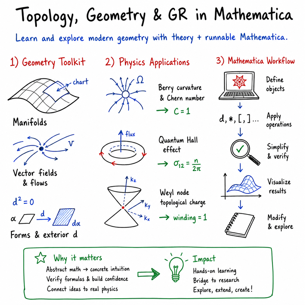
Abstract: This book is a self-contained, tutorial introduction to topology, differential geometry, and general relativity for students and researchers in physics. Its distinguishing feature is a Mathematica-based approach that makes abstract constructions concrete through explicit, runnable notebooks and worked examples. A key contribution is a large collection of original Mathematica notebooks, written by the authors themselves, that let readers run, verify, and extend every demonstration. The first part covers point-set topology, topological spaces, continuity of maps, homotopy, and the fundamental group with applications that highlight the role of topology in modern physics. The second and largest part develops differential geometry from the ground up: manifolds, tangent and dual spaces, vector fields, pullbacks and pushforwards, Lie brackets and Lie algebras, local flows, and the Lie derivative. It then treats tensors, differential forms, the exterior derivative, volume forms, the metric tensor, and Hodge duality, emphasizing coordinate-free formulations and their computational realization. These tools are applied to Maxwell's equations in the language of forms and the generalized Stokes theorem, while Lie groups, fiber bundles, connections, and curvature bridge geometry and gauge-theoretic physics. The final part uses this framework to present general relativity, computing curvature tensors and field equations for standard spacetimes with dedicated Mathematica packages. Throughout, the book balances mathematical rigor with hands-on computation, enabling readers both to understand the theory and to reproduce every result themselves.
Paper Prompts
Sign up for free to create and run prompts on this paper.
Top Community Prompts
Explain it Like I'm 14
1. Brief overview
This work is a teaching book, rather than a study reporting one new experiment. Its purpose is to introduce students to three important areas of mathematics used in physics:
- Topology: the study of shapes and spaces, especially properties that do not change when a shape is stretched or bent.
- Differential geometry: the study of curved spaces using calculus.
- General relativity: Einstein’s theory explaining gravity as the bending of space and time.
A special feature is that the authors use Mathematica, a computer program for mathematics, to demonstrate the ideas. Readers can run the examples, check the calculations, and experiment with them.
2. Main objectives and questions
The book aims to help beginners answer questions such as:
- What does it mean for two shapes to be “the same” if one can be stretched into the other?
- How can we describe curved surfaces, such as a sphere or a doughnut-shaped surface?
- How can we measure distances and angles on curved spaces?
- How do mathematical ideas about curves and spaces help explain electricity, magnetism, and gravity?
- How can computers perform difficult calculations with tensors, curvature, and Einstein’s equations?
- Can students use Mathematica to explore these ideas instead of only reading abstract formulas?
The authors also want to make subjects that are often difficult for beginners more concrete and understandable.
3. Research and teaching approach
Because this is a tutorial book, the authors do not use surveys, laboratory experiments, or measurements from nature. Instead, they combine mathematical explanations with computer demonstrations.
Mathematical explanations
The book begins with topology. Topology studies features of objects that remain unchanged when the objects are smoothly stretched or deformed. For example, a coffee mug and a doughnut are considered similar in topology because each has one hole. A sphere has no hole, so it is topologically different.
The authors introduce ideas such as:
- Topological spaces: sets of objects together with rules describing which parts count as “open.”
- Continuity: a function is continuous if it does not make sudden jumps.
- Connectedness: whether a space is in one piece.
- Compactness: a technical idea describing spaces that can be covered in a controlled way by a finite number of smaller pieces.
- Homotopy: smoothly changing one shape or loop into another without cutting or gluing.
- Fundamental group: a way of recording which loops can or cannot be shrunk to a point.
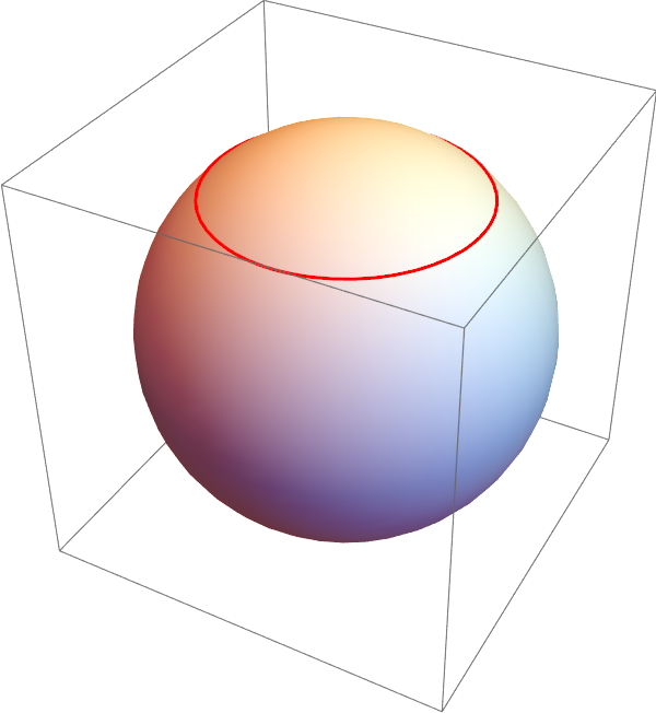
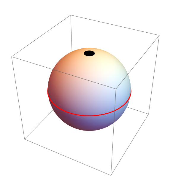
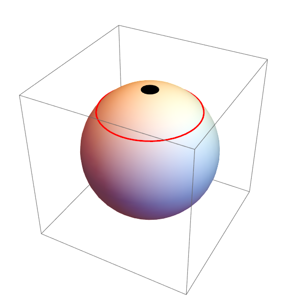
For example, imagine drawing a loop on a rubber sheet. On a flat sheet, the loop can usually be shrunk to a point. On the surface of a doughnut, some loops cannot be shrunk because they wrap around the hole. The fundamental group helps describe this difference.
The book then develops differential geometry, which uses calculus to study curved spaces. It explains:
- Manifolds: spaces that may be curved overall but look flat when viewed closely, like Earth appearing flat when standing in a small area.
- Tangent vectors: arrows showing directions along a curved surface.
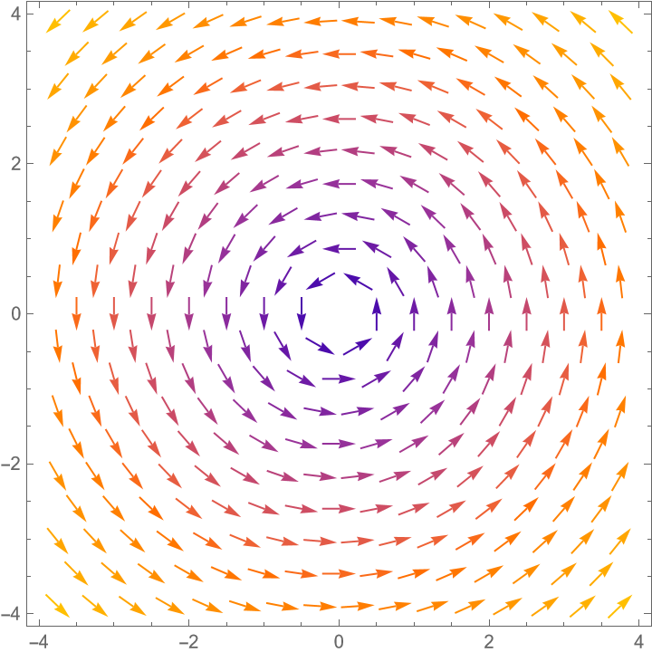
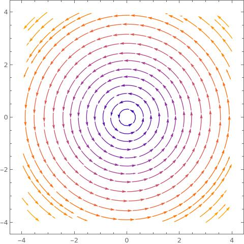
- Vector fields: arrows placed at many points, like a map showing wind direction.
- Tensors: mathematical objects that describe physical quantities in a way that works in different coordinate systems.
- Differential forms: useful mathematical tools for describing quantities that can be integrated over curves and surfaces.
- Metric tensors: rules for measuring distances and angles.
- Curvature: a measure of how much a surface or space bends.
Finally, the book applies these tools to physics, including:
- Maxwell’s equations for electricity and magnetism.
- Lie groups and symmetries.
- Fiber bundles and connections, which are useful in modern physics.
- General relativity, including black holes and expanding-universe models.
Use of Mathematica
The authors provide many runnable Mathematica notebooks. A notebook is like a digital worksheet containing explanations, computer code, and results.
For instance, a simple program checks whether a collection of subsets satisfies the rules needed to be a topology. Other notebooks:
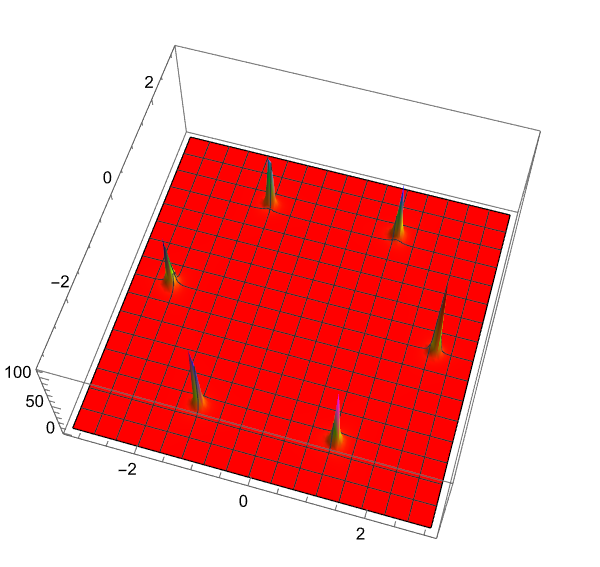
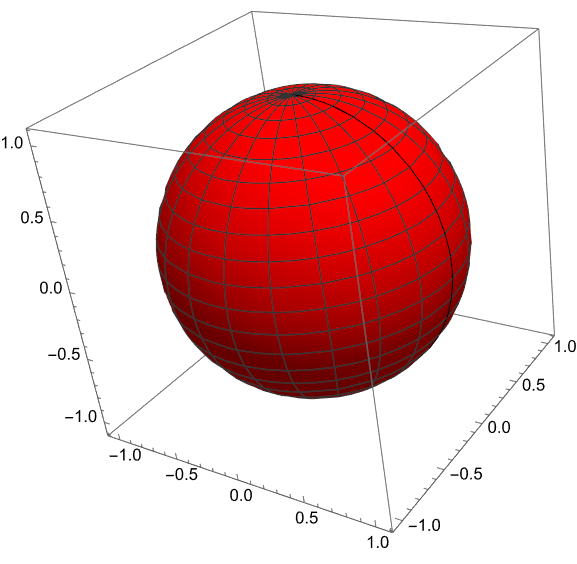
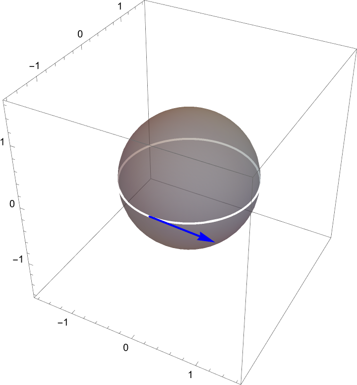
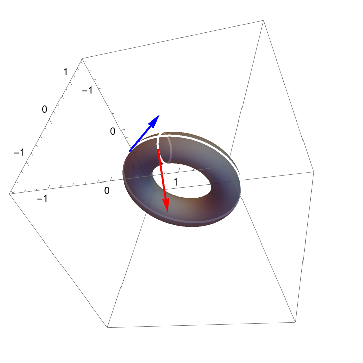
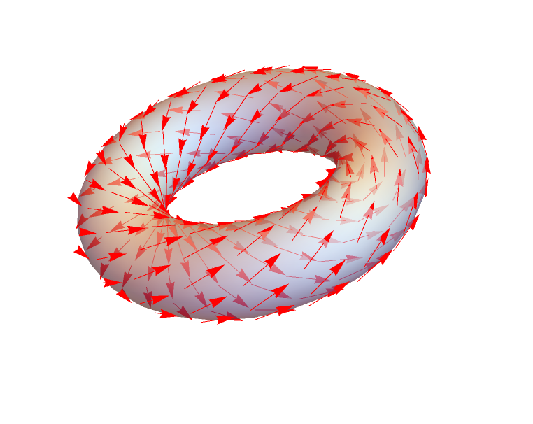
- Draw vector fields on spheres and doughnuts.
- Show loops being continuously deformed.
- Calculate curvature.
- Work with matrices and tensors.
- Derive properties of the Schwarzschild solution, which describes the space around a non-rotating spherical object such as an idealized black hole.
- Explore the Friedmann–Robertson–Walker model used to describe the large-scale universe.
The computer acts like a very fast calculator and checking partner. It does not replace understanding, but it helps students see how abstract definitions produce actual results.
4. Main findings and results
Since the book is educational, its “results” are mainly the mathematical conclusions and demonstrations it develops.
Important mathematical results
The book shows that:
- A topology must obey specific rules involving empty sets, unions, and intersections.
- Continuity can be defined in a very general way using open sets. This general definition becomes the familiar idea that a function has no sudden jumps.
- A space can be connected or disconnected depending not only on its points but also on the chosen topology.
- Loops can be grouped together when they can be smoothly deformed into one another.
- These groups of loops, called fundamental groups, reveal important information about the shape of a space.
- Spaces that can be smoothly transformed into one another have the same basic topological information.
- If a complicated space can be continuously shrunk to a simpler part, studying the simpler part can reveal properties of the original space.
- Curved spaces can be studied using coordinate systems, vectors, tensors, forms, metrics, and curvature.
- The mathematical language of differential geometry provides a natural way to express Maxwell’s equations and general relativity.
Why these results matter
These ideas are important because ordinary geometry is not enough for many modern physics problems. A flat graph or a simple three-dimensional coordinate system cannot fully describe:
- The curved surface of a planet.
- The shape of space around a black hole.
- The expanding universe.
- Symmetries in particle physics.
- Electromagnetic fields and gauge theories.
The book’s computer examples are also important because they allow readers to reproduce the calculations themselves. Instead of accepting a formula as something mysterious, students can change the inputs, run the code, and observe what happens.
5. Implications and potential impact
The main impact of this work is educational. It provides a bridge between abstract mathematics and practical computer exploration.
For students, the book may:
- Make difficult ideas easier to visualize.
- Show how mathematical definitions are used in real physics.
- Build confidence with symbolic computation.
- Provide a starting point for research projects.
- Help connect classroom mathematics with topics such as black holes, cosmology, electromagnetism, and quantum physics.
For teachers, the notebooks can be used as demonstrations, homework activities, or starting points for student projects. For researchers, the examples may be adapted for more advanced calculations.
In simple terms, the book teaches that the shape and structure of space are deeply connected to the laws of physics. It also shows that computers such as Mathematica can help students explore this connection. The work does not present one single new scientific discovery; instead, its contribution is to make powerful mathematical and physical ideas more accessible, interactive, and usable.
Knowledge Gaps
Knowledge gaps, limitations, and open questions
- The supplied text is incomplete: it ends during the first homotopy example, so the treatment and conclusions for later chapters—especially differential geometry, gauge theory, fiber bundles, curvature, and general relativity—cannot be assessed.
- The book does not report systematic testing with its intended undergraduate or graduate audience; its claims about improving accessibility, conceptual understanding, or Mathematica proficiency remain empirically unvalidated.
- No comparative study evaluates whether the Mathematica-based approach is more effective than conventional lecture notes, textbooks, numerical tools, or alternative computer-algebra systems.
- The learning prerequisites are not operationally specified: the text does not define the expected level of mathematical maturity, programming experience, physics background, or prior exposure to topology and geometry.
- The Mathematica notebooks are described as runnable and tested with Mathematica 12.3, but the paper does not provide systematic information about testing across operating systems, later Mathematica versions, package versions, or hardware environments.
- The long-term reproducibility of examples relying on external packages such as
Ricci,DifferentialForms,Difform, andEDCRGTCis uncertain because compatibility, maintenance status, installation procedures, and dependency management are not systematically documented. - The notebooks are not accompanied by documented automated tests or independent verification procedures that would establish the correctness of their symbolic outputs.
- The computational treatment appears largely example-driven; it does not establish general algorithms for automatically representing arbitrary topological spaces, manifolds, atlases, transition maps, bundles, or geometric structures.
- The finite-set topology code is not shown to scale beyond very small sets, and no complexity analysis or practical limit is given for enumerating subsets and candidate topologies.
- The implementation of
IsTopologyQand related code is not evaluated against edge cases such as duplicate representations, nested or symbolic sets, infinite sets, nonstandard equality behavior, or malformed inputs. - The text does not clarify how Mathematica represents genuinely infinite topological spaces or verifies properties involving arbitrary unions, open covers, compactness, or continuity that cannot be exhaustively enumerated.
- Several mathematical arguments are stated rather than fully proved, including the Heine–Borel theorem, the group structure of the fundamental group, base-point independence, and invariance under homotopy equivalence; the extent to which this compromises the claimed self-contained character is not discussed.
- The distinction between rigorous symbolic verification and illustrative computation is not sufficiently developed; successful execution of a notebook does not by itself establish a theorem for all admissible mathematical objects.
- The treatment of homotopy and the fundamental group does not indicate how non-path-connected spaces, changing base points, or groupoids are handled.
- Higher homotopy groups, homology and cohomology, covering spaces, van Kampen’s theorem, and other tools needed for broader topological analysis are not addressed, leaving unclear how far the proposed framework extends beyond .
- The selected physical applications are limited relative to the stated scope: the paper does not explore substantial applications in condensed matter, quantum field theory, cosmology, quantum information, or modern geometric methods such as characteristic classes and index theory.
- The relationship between the abstract mathematical definitions and the concrete Mathematica data structures is not formalized, making it unclear whether coordinate-dependent implementations preserve coordinate-free concepts in all cases.
- No analysis is provided of numerical stability, symbolic-expression growth, computation time, or memory requirements for the differential-geometric and general-relativistic examples.
- The behavior of the computational methods near coordinate singularities, degenerate metrics, nontrivial global topologies, boundaries, and singular spacetime geometries is left unresolved.
- The paper does not establish whether the packages correctly handle global manifold structure rather than only local coordinate calculations; issues involving chart compatibility, transition functions, and global tensor fields require further validation.
- The treatment of general relativity appears centered on standard analytic spacetimes such as Schwarzschild and FRW, leaving the performance and correctness of the workflow for less symmetric, numerically generated, or physically realistic spacetimes unexplored.
- There is no systematic comparison between the Mathematica implementations and independent tools such as SageMath, Maple, SymPy, xAct, Cadabra, or numerical relativity software.
- The accessibility of the resource is limited by dependence on proprietary Mathematica, but the paper does not investigate open-source alternatives or provide language-independent representations of the examples.
- The pedagogical material does not appear to include structured exercises with solutions, learning assessments, error diagnosis, or guidance for instructors using the notebooks in formal courses.
- The role of artificial-intelligence tools in preparing or supporting the material is acknowledged, but there is no discussion of how AI-generated content was verified, what errors were detected, or how AI use should be integrated responsibly into student learning.
- The repository’s sustainability is not evaluated: the paper does not specify contribution guidelines, issue tracking, versioning policy, archival strategy, or procedures for updating notebooks as Mathematica and external packages evolve.
- The text contains apparent notation, formatting, and code inconsistencies in the supplied version—such as missing or corrupted symbols and malformed function arguments—but does not document an errata process or assess their impact on reader comprehension and reproducibility.
- The resource’s effectiveness for researchers, rather than beginners, remains untested; it is unclear whether the notebooks can be adapted efficiently to research-scale calculations or primarily serve demonstrative purposes.
- No framework is provided for extending the notebooks to other physical theories, alternative signatures, supersymmetric or higher-dimensional geometries, noncommutative geometry, or computationally intensive models.
Practical Applications
Immediate Applications
- Physics education and computational laboratories — Academia
- Use the book and its runnable Mathematica notebooks as a modular curriculum for undergraduate or graduate courses in mathematical physics, differential geometry, general relativity, gauge theory, or theoretical condensed matter.
- Instructors can assign notebooks on manifolds, tangent spaces, differential forms, Lie groups, Maxwell equations, geodesics, and curvature as laboratory exercises alongside formal lectures.
- Potential workflow: students read a short theoretical section, execute the corresponding notebook, modify parameters or coordinate systems, and submit both symbolic calculations and visualizations.
- Dependencies: access to Mathematica 12.3 or a compatible Wolfram environment; installation and maintenance of external packages such as
Ricci,DifferentialForms,Difform, andEDCRGTC; instructor review is needed because some examples are pedagogical rather than production-grade software.
- Reproducible verification of textbook calculations — Academia and research
- Researchers and students can use the notebooks to reproduce standard calculations involving Christoffel symbols, Riemann and Ricci tensors, scalar curvature, geodesics, Schwarzschild spacetime, and Friedmann–Robertson–Walker metrics.
- This provides a practical checking layer for lecture notes, theses, research drafts, and symbolic derivations.
- Potential product or workflow: a version-controlled repository of notebooks accompanying a paper, with automated execution and comparison of expected outputs.
- Dependencies: symbolic expressions can become computationally expensive; results must be checked for coordinate conventions, index ordering, metric signature, assumptions, and package-version differences.
- Interactive visualization of abstract geometric concepts — Education and scientific communication
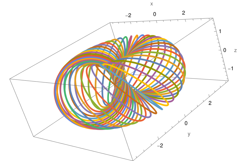
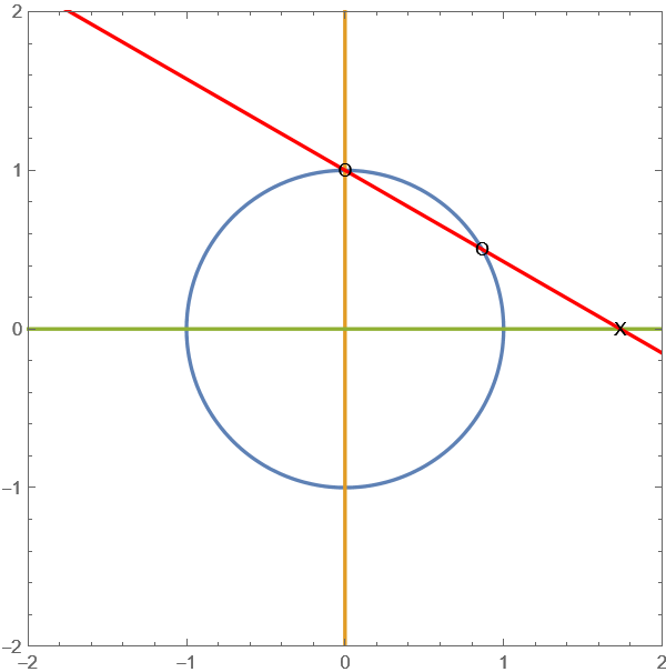
- The notebooks can support demonstrations of stereographic projection, vector fields, integral curves, homotopies, the Hopf fibration, Berry curvature, and geometric structures on spheres and tori.
- These visualizations can be integrated into classroom presentations, online courses, public lectures, or interactive teaching materials to make otherwise abstract constructions more accessible.
- Dependencies: visualizations generally illustrate selected finite-dimensional examples and should not be interpreted as complete representations of the underlying mathematical spaces or physical systems.
- Symbolic derivation of electromagnetic identities — Electromagnetism and engineering education
- The differential-form treatment of Maxwell equations and the generalized Stokes theorem can be used to verify coordinate-free formulations, translate between tensor and vector-calculus descriptions, and test equations in different coordinate systems.
- Potential workflow: formulate electromagnetic fields as differential forms, apply the exterior derivative and Hodge dual, and verify local or integral conservation laws symbolically.
- Dependencies: practical engineering deployment would require constitutive relations, boundary conditions, material models, numerical discretization, and experimental validation; the paper primarily provides educational symbolic examples.
- Exploration of geometric phases and topological structures — Condensed matter and quantum-physics research
- The Berry-phase and Berry-curvature notebooks can serve as starting points for analyzing parameter-dependent quantum systems, band structures, geometric phases, and topological effects in condensed matter.
- Researchers can adapt the examples to compute curvature over a model parameter space and visualize it as an effective “magnetic field.”
- Dependencies: meaningful physical predictions require a correctly specified Hamiltonian, gauge-consistent eigenvectors, treatment of degeneracies, appropriate parameter sampling, and comparison with established numerical or experimental methods.
- Rapid prototyping of geometry calculations — Theoretical physics and software-assisted research
- The combination of Mathematica’s symbolic capabilities with the listed differential-geometry packages can be used to prototype calculations before implementing them in larger numerical or high-performance-computing systems.
- Examples include testing candidate metrics, deriving curvature tensors, exploring Lie-algebra relations, and checking connections and curvature.
- Dependencies: notebooks are not presented as optimized software libraries, and symbolic results may not scale to high-dimensional, discretized, or data-intensive problems.
- Open educational resource development — Universities and public research institutions
- The freely available lecture material, GitHub notebooks, and open-source auxiliary packages can be reused to create localized course modules, student projects, laboratory manuals, and supplementary material for physics programs.
- Dependencies: reuse should respect repository and package licenses, preserve attribution, and account for future incompatibilities with Mathematica or external packages.
- Personal learning and self-study — Daily life and professional development
- Learners can use the notebooks as an interactive route into topology, differential geometry, and relativity, experimenting with code rather than relying only on static equations.
- The notebook format supports a cycle of explanation, execution, modification, and immediate feedback.
- Dependencies: users still need foundational mathematics and physics; symbolic software can produce formally valid output without explaining whether a model or assumption is physically appropriate.
Long-Term Applications
- A reusable symbolic differential-geometry toolkit — Scientific software
- The examples could be refactored into a unified, documented library for manifolds, coordinate charts, tensors, differential forms, Lie derivatives, connections, curvature, and spacetime metrics.
- Such a tool could offer standardized data structures, validation of coordinate transformations, automatic consistency checks, and export to numerical solvers or code-generation systems.
- Dependencies: substantial software engineering is required, including performance optimization, unit testing, interoperability among the currently separate packages, version control, and clear treatment of conventions.
- Automated research workflows for general relativity — Astrophysics and gravitational physics
- The curvature and geodesic calculations could become components of systems that automatically derive field equations for proposed metrics, test symmetry assumptions, calculate observables, and generate numerical initial conditions.
- Possible applications include exploratory models of compact objects, cosmological spacetimes, gravitational lensing, and wave propagation.
- Dependencies: symbolic calculations must be combined with numerical relativity, physically justified matter models, stable numerical methods, observational constraints, and rigorous validation. The book itself does not establish predictive accuracy for new astrophysical models.
- Computer-assisted gauge-theory and field-theory modeling — High-energy physics
- The treatment of Lie groups, fiber bundles, connections, curvature, differential forms, and Hodge duality could support software for constructing and checking gauge-theoretic models.
- Potential tools: model-building assistants that verify group representations, connection transformations, curvature forms, Bianchi identities, and coordinate-free field equations.
- Dependencies: further work is needed to handle large representations, quantum corrections, anomalies, constraints, and integration with existing high-energy-physics packages.
- Topological analysis of quantum materials — Condensed matter
- The Berry-curvature and homotopy examples could be extended into pipelines for calculating topological invariants, identifying phase transitions, and screening candidate Hamiltonians or materials.
- A future workflow could combine symbolic derivations with numerical band-structure data and visualization dashboards for researchers.
- Dependencies: realistic materials require large-scale numerical calculations, disorder and interaction effects, gauge-invariant discretization, experimental calibration, and robust handling of band crossings and finite-resolution data.
- Geometric modeling in robotics and control — Robotics
- The manifold, tangent-vector, Lie-group, Lie-bracket, local-flow, and geodesic material could inform future educational or software tools for modeling robot orientations, rigid-body motion, configuration spaces, and nonlinear control systems.
- For example, rotations represented through or could be incorporated into trajectory-planning and state-estimation algorithms without treating orientations as ordinary Euclidean vectors.
- Dependencies: the paper does not develop robotics algorithms or address sensor noise, real-time constraints, collision avoidance, or embedded implementation. Translation from symbolic demonstrations to deployed robotics would require numerical and experimental development.
- Structure-preserving numerical simulation — Engineering and computational science
- The coordinate-free emphasis on differential forms, exterior derivatives, metrics, Hodge duality, and Stokes’ theorem could contribute to numerical methods that preserve geometric or physical structure, particularly for electromagnetism and continuum models.
- Potential products: finite-element or discrete-exterior-calculus software that automatically derives compatible discretizations and checks conservation identities.
- Dependencies: this requires discretization theory, convergence and stability analysis, mesh handling, boundary-condition support, and benchmarking against established solvers.
- Interactive digital textbooks and intelligent tutoring systems — Education technology
- The book’s integration of exposition, code, visualization, and exercises could be expanded into adaptive learning platforms that detect errors in symbolic calculations, generate parameter variations, and provide stepwise hints.
- AI-assisted interfaces could explain Mathematica syntax or connect a failed computation to the relevant mathematical definition.
- Dependencies: automated feedback must distinguish programming errors from mathematical misconceptions; generated explanations require expert validation, and access to proprietary Mathematica functionality may limit deployment.
- Policy and research-infrastructure support for reproducible computational science — Research policy
- The paper’s notebook-centered approach supports policies requiring executable supplements, versioned computational artifacts, and open repositories for symbolic calculations in physics.
- Funding agencies, journals, and universities could encourage or require notebooks that reproduce central derivations and document software versions and dependencies.
- Dependencies: reproducibility requires long-term repository preservation, license-compatible software, environment capture, executable testing, and standards for acceptable symbolic verification.
- Cross-platform and open-source alternatives — Scientific-computing ecosystems
- The material could be ported from Mathematica to open-source environments such as Python/SymPy, SageMath, or Julia, making the instructional and computational methods more accessible.
- A cross-platform implementation could also connect symbolic geometry to numerical libraries, visualization tools, and high-performance computing.
- Dependencies: equivalent support for tensor calculus, differential forms, Lie groups, and interactive notebooks must be developed and validated; numerical and symbolic outputs may differ because of convention and simplification rules.
- Geometry-informed data analysis — Finance, healthcare, and machine learning
- In the longer term, the manifold and differential-geometric concepts could provide educational and methodological foundations for analyzing data that naturally lie on non-Euclidean spaces, such as covariance matrices, rotations, shape spaces, or constrained physical states.
- Possible applications include geometric machine learning, medical-shape analysis, and manifold-valued time series.
- Dependencies: these applications are not demonstrated by the paper and would require new statistical theory, domain-specific validation, scalable algorithms, and evidence that geometric representations improve decision-making over established methods.
Glossary
- Bijection: A function that is both one-to-one and onto. “If a map is one-to-one and onto, i.e. a \db{bijection}”
- Closed set: A set whose complement is open in the relevant topological space. “A set is \db{closed} if its complement in also written or as , is open.”
- Compactness: The property that every open cover has a finite subcover. “Inspired by this, we define \db{compactness} as follows:”
- Connectedness: The property of a topological space that prevents it from being partitioned into two disjoint nonempty open sets. “Another central idea in topology is that of \db{connectedness}”
- Contractible: Describes a space that can be continuously deformed to a point. “If a point is a deformation retraction of , is said to be contractible.”
- Contraction: A homotopy that continuously deforms a space to a point. “The homotopy connecting and is called a contraction.”
- Continuous map: A map for which the inverse image of every open set is open. “A map is \db{continuous} if given any open set its inverse image (or pre-image, what it is an image of) is open”
- Deformation retract: A subspace to which the larger space can be continuously deformed while keeping the subspace fixed. “A subset of a topological space is a \db{deformation retract}”
- Disconnected: Describes a space that is the union of two disjoint nonempty open subsets. “then the topological space is called \db{disconnected}.”
- Discrete topology: The topology containing every subset of the underlying set as an open set. “The \db{discrete} topology on a set = \{ A\,|\, A\subset\}, consists of all subsets of ”
- Exterior differential calculus: A calculus based on differential forms and their exterior derivatives. “EDC {paper_content} RGTC: Exterior Differential Calculus and Riemannian Geometry {paper_content} Tensor Calculus”
- Finite subcover: A finite collection selected from an open cover that still covers the original set. “a finite subcover is defined as a finite collection of open sets from an open cover of a topological space that still covers the entire space.”
- Fundamental group: The group of homotopy classes of loops based at a point in a topological space. “the collection of all distinct homotopy classes of loops in based at is , called the fundamental group or first homotopy group of at .”
- Hausdorff space: A topological space in which every pair of distinct points has disjoint neighbourhoods. “A topological space is said to be \db{Hausdorff} if two distinct points have disjoint neighbourhoods.”
- Heine–Borel theorem: A theorem stating that every open cover of a closed and bounded subset of Euclidean space has a finite subcover. “The Heine-Borel Theorem states that every open cover of a closed bounded subset of (in the usual topology) admits a finite subcover.”
- Homeomorphism: A bijective continuous map whose inverse is also continuous. “If a map is one-to-one and onto, i.e. a \db{bijection}, and both and are continuous, is called a \db{homeomorphism}”
- Homeomorphic: Describes two topological spaces related by a homeomorphism. “we say that and are \db{homeomorphic}.”
- Homomorphism: A map between groups that preserves the group operation, identity, and inverses. “A map that preserves the group multiplication ”
- Homotopy: A continuous deformation between maps, particularly between loops. “This leads to the notion of \db{homotopy}, which is an equivalence relation.”
- Homotopy class: The collection of objects equivalent under homotopy. “Equivalence relations partition a collection of objects into disjoint classes, called equivalence classes.”
- Homotopy type: A relationship between spaces connected by maps whose compositions are homotopic to the identity maps. “Two topological spaces and are of the same \db{homotopy type}”
- Inverse loop: A loop traversed in the reverse direction. “The inverse of a loop is defined by for .”
- Isomorphism: A bijective homomorphism between algebraic structures. “If the homomorphism is bijective, it is called an isomorphism.”
- Loop: A path whose initial and terminal points coincide. “A closed path or \db{loop} in based at is a path for which .”
- Neighbourhood: A set containing an open set around a specified point. “A \db{neighbourhood} of is a set containing an open neighbourhood of .”
- Open cover: A collection of open sets whose union contains the space or set under consideration. “For a topological space , if , then is called an \db{open cover}.”
- Open set: A member of a topology; informally, a set regarded as having no boundary points within the space. “A \db{topological space} is a set together with a collection of subsets called \db{open sets}”
- Path connected: Describes a space in which every pair of points can be joined by a continuous path. “If a path between any two points in , is called path connected.”
- Product loop: A loop formed by traversing one loop followed by another. “the \db{product loop} is defined by”
- Retract: A subspace onto which the larger space admits a map acting as the identity on the subspace. “A \db{retract} of a topological space is a subspace of ”
- Retraction: A map from a space to a subspace that fixes every point of the subspace. “such that a continuous map which preserves the position of all points in that subspace”
- Subcover: A subcollection of a cover that still covers the same set. “We note that a subcover is a subset of an existing cover of a set that still covers the original set”
- Topological invariant: A property preserved under topological equivalence, such as homeomorphism. “This corollary establishes the fundamental group as a topological invariant.”
- Topological space: A set equipped with a collection of subsets satisfying the topology axioms. “A \db{topological space} is a set together with a collection of subsets”
- Topology: A collection of subsets satisfying closure conditions under finite intersections and arbitrary unions. “It is the pair which is, precisely speaking, a topological space, or alternatively a \db{space with topology}.”
- Trivial topology: The topology containing only the empty set and the entire underlying set. “The \db{trivial} topology on ”
- Tuple: An ordered collection of values, used in the paper to specify index ranges in Mathematica. “The second element is a tuple, which denotes that goes from 1 to .”
- User-defined function: A function created by the programmer rather than supplied by the language. “\item User-defined function: Mathematica allows users to write their own code for a custom function.”
- Van Kampen-type fundamental-group reasoning: Reasoning involving the algebraic structure formed by loop classes; the supplied excerpt introduces the fundamental group but does not explicitly use van Kampen’s theorem. “the fundamental group or first homotopy group of at .”