A metric on $S^2 \times S^2$ with positive sectional curvature

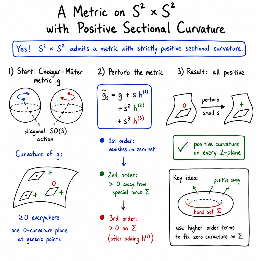
Abstract: We construct a metric on $S² \times S<sup>2$ with positive sectional curvature. Starting from the standard metric on $S² \times S<sup>2$, we first perform a Cheeger deformation. The resulting metric has nonnegative sectional curvature. We refer to it as a Cheeger-Müter metric. We then consider a suitable third order perturbation of this Cheeger-Müter metric and show that the perturbed metrics have positive sectional curvature. The proof requires various calculations, some of which have been carried out with the help of MATHEMATICA. The MATHEMATICA code is attached to this submission.

• The paper proves that S² × S² admits a Riemannian metric with strictly positive sectional curvature, resolving a longstanding four-dimensional existence problem.
• The authors begin with the nonnegatively curved Cheeger–Müter metric and use a carefully designed third-order perturbation whose second-order effects remove most degeneracies and whose third-order correction eliminates the remaining torus.
• The construction preserves no nontrivial continuous symmetry, consistent with the Hsiang–Kleiner obstruction, and combines geometric estimates, perturbative minimization, and computer-assisted symbolic calculations to establish global positivity.

The paper establishes the existence of a Riemannian metric with strictly positive sectional curvature on $S^2 \times S^2$. This answers a classical existence problem in dimension four while respecting the substantial obstruction imposed by symmetry: by the theorem of Hsiang and Kleiner, a positively curved four-manifold with a nontrivial Killing field must be homeomorphic to $S^4$ or $\mathbb{CP}^2$. Consequently, a positively curved metric on $S^2 \times S^2$ cannot retain a nontrivial continuous isometry group. The construction therefore begins with a highly symmetric nonnegatively curved metric and destroys its zero-curvature planes through carefully designed perturbations (2608.19068).

Geometric starting point

Let $M=S^2\times S^2$, equipped initially with the standard product metric. Applying a Cheeger deformation with respect to the diagonal $SO(3)$-action produces the Cheeger–Müter metric. The authors work with the deformation parameter $t=1$, after a normalization by a factor of $2$. On the dense open subset

$$M_{\mathrm{generic}}=M\setminus(\Delta_+\cup\Delta_-),$$

where $\Delta_+$ and $S^4$0 are the diagonal and anti-diagonal, respectively, they identify the manifold with $S^4$1.

In these coordinates, the normalized background metric is

$S^4$2

The Cheeger–Müter metric has nonnegative sectional curvature. More precisely, at every point of $S^4$3, exactly one two-plane has zero sectional curvature, while all other two-planes have strictly positive sectional curvature. The zero-curvature planes form a smooth four-dimensional submanifold $S^4$4 of the eight-dimensional Grassmannian of two-planes in $S^4$5. This structure is essential: the perturbation need not increase curvature uniformly at first order in every direction, but only needs to remove the degeneracy along $S^4$6.

The appendix supplies a quantitative estimate of the form

$S^4$7

for some $S^4$8, where $S^4$9 denotes the unnormalized curvature numerator on the space of two-planes. This quadratic lower bound is the coercive component of the argument. It reduces the global positivity problem to analyzing the perturbation near the zero-curvature locus.

The perturbative mechanism

The metric is constructed as a third-order perturbation

$\mathbb{CP}^2$0

The role of the three orders is sharply differentiated. The first-order perturbation is selected so that the curvature variation vanishes on the distinguished zero-curvature planes. The second-order perturbation then makes the minimized sectional curvature nonnegative, with strict positivity except along a special two-dimensional torus. The third-order term finally removes the remaining degeneracy on that torus.

To formalize minimization over nearby two-planes, the authors introduce an abstract framework. If a smooth function $\mathbb{CP}^2$1 has a nonnegative zeroth-order term vanishing quadratically along $\mathbb{CP}^2$2, and its first-order term also vanishes there, then minimization over $\mathbb{CP}^2$3 yields an expansion

$\mathbb{CP}^2$4

The coefficients incorporate the displacement of the minimizing plane. In particular, $\mathbb{CP}^2$5 is not simply the pointwise second-order curvature coefficient: it includes a negative-completion term arising from the first variation in the transverse plane variables. This is the finite-dimensional analogue of eliminating the transverse variables by the implicit function theorem.

The manifold version shows that if $\mathbb{CP}^2$6 is bounded below by a nonnegative function $\mathbb{CP}^2$7 and $\mathbb{CP}^2$8 is strictly positive on the zero set of $\mathbb{CP}^2$9, then the minimized curvature is positive for sufficiently small positive $S^2 \times S^2$0. The conclusion remains valid even when the local coordinate description applies only on a dense open subset of the zero-curvature locus. This density argument is what allows the authors to control the singular-looking regions near $S^2 \times S^2$1 and $S^2 \times S^2$2.

First- and second-order curvature analysis

The curvature tensor of a perturbed metric is expanded using differential operators $S^2 \times S^2$3, $S^2 \times S^2$4, and $S^2 \times S^2$5, respectively linear, bilinear, and trilinear in the perturbation tensors:

$S^2 \times S^2$6

$S^2 \times S^2$7

and

$S^2 \times S^2$8

The authors encode the curvature of planes near the zero-curvature plane by four transverse parameters. Projection operators $S^2 \times S^2$9, $M=S^2\times S^2$0, and $M=S^2\times S^2$1 extract the curvature value, its first derivatives, and its transverse Hessian. If $M=S^2\times S^2$2 and $M=S^2\times S^2$3, the displacement of the minimizing plane is determined by

$M=S^2\times S^2$4

The minimized second-order coefficient is then

$M=S^2\times S^2$5

The first-order tensor $M=S^2\times S^2$6 is assembled from four globally smooth components. Two components, $M=S^2\times S^2$7 and $M=S^2\times S^2$8, generate the principal second-order curvature increase; two additional components, weighted by parameters $M=S^2\times S^2$9 and $SO(3)$0, are used to control the third-order term. The second-order tensor $SO(3)$1 contains ten components, with coefficients involving trigonometric polynomials and convergent Fourier series. The elaborate expressions are not merely coordinate artifacts: they solve the cancellation equations required to eliminate unfavorable second-order terms while preserving smoothness across the exceptional sets.

The first-order minimized curvature vanishes:

$SO(3)$2

This is a deliberate cancellation, not a failure of the perturbation. It reflects the fact that the remaining zero-curvature planes are sufficiently degenerate that a first-order correction cannot provide the required uniform positivity without creating incompatible terms elsewhere.

The main second-order estimate is

$SO(3)$3

on $SO(3)$4, provided $SO(3)$5 is sufficiently small. The coefficient contributed by the principal components is

$SO(3)$6

which is strictly positive. The error terms involving $SO(3)$7 are controlled by choosing $SO(3)$8 in a sufficiently small neighborhood of zero.

The factor on the right-hand side is the squared component of the normalized vector

$SO(3)$9

orthogonal to $t=1$0. Thus, $t=1$1 is strictly positive away from the torus

$t=1$2

On $t=1$3, one has $t=1$4. The implication is that second-order positivity resolves the degeneracy in every direction except one geometrically prescribed two-dimensional family. The perturbation has therefore reduced the problem from a four-dimensional zero-curvature locus in the Grassmannian to a two-dimensional residual set in the base manifold.

The third-order correction

The authors next prove that $t=1$5 restricted to $t=1$6 extends smoothly across the closure to all of $t=1$7. This extension is important because the coordinate representation of $t=1$8 degenerates near $t=1$9.

The parameters $2$0 are chosen so that the restriction of $2$1 to $2$2 is not identically zero. The proof uses the fact that this restriction is a polynomial in $2$3 and $2$4. The coefficient of the monomial $2$5 is computed explicitly and is nonzero; the paper reports the value

$2$6

Hence the set of parameter pairs for which $2$7 is open and dense in $2$8. This is a strong structural statement: the third-order nondegeneracy is generic within the two-parameter family used by the construction, rather than dependent on an isolated numerical choice.

However, nonvanishing alone does not imply a uniform sign on $2$9. The authors address this by subtracting the average-free component of $$M_{\mathrm{generic}}=M\setminus(\Delta_+\cup\Delta_-),$$0. Let $$M_{\mathrm{generic}}=M\setminus(\Delta_+\cup\Delta_-),$$1 solve

$$M_{\mathrm{generic}}=M\setminus(\Delta_+\cup\Delta_-),$$2

for a nonzero constant $$M_{\mathrm{generic}}=M\setminus(\Delta_+\cup\Delta_-),$$3, where $$M_{\mathrm{generic}}=M\setminus(\Delta_+\cup\Delta_-),$$4 is the Laplacian induced by $$M_{\mathrm{generic}}=M\setminus(\Delta_+\cup\Delta_-),$$5. Extending $$M_{\mathrm{generic}}=M\setminus(\Delta_+\cup\Delta_-),$$6 smoothly to $$M_{\mathrm{generic}}=M\setminus(\Delta_+\cup\Delta_-),$$7 and setting

$$M_{\mathrm{generic}}=M\setminus(\Delta_+\cup\Delta_-),$$8

changes the third-order minimized coefficient on $$M_{\mathrm{generic}}=M\setminus(\Delta_+\cup\Delta_-),$$9 from $\Delta_+$0 to the constant $\Delta_+$1. This use of a conformal third-order correction is precise: it removes the oscillatory component of the third-order curvature while retaining its nonzero average.

If $\Delta_+$2, positive values of $\Delta_+$3 are used; if $\Delta_+$4, the sign of $\Delta_+$5 is reversed. Thus the construction does not require prescribing the sign of the perturbation parameter in advance.

Global positivity

The final argument applies the abstract minimization theorem to the normalized curvature numerator on the Grassmannian of two-planes. The zeroth-order curvature is quadratically bounded below away from $\Delta_+$6, while the first-order term vanishes on $\Delta_+$7. The second-order coefficient satisfies a lower bound proportional to

$\Delta_+$8

where $\Delta_+$9 is the unit vector determining the zero-curvature plane $S^4$00. The zero set of $S^4$01 consists precisely of the planes over $S^4$02 corresponding to the vertical direction $S^4$03.

On the open dense subset $S^4$04, the second-order coefficient is positive wherever $S^4$05. Along $S^4$06, the third-order coefficient equals the positive constant $S^4$07 after the final correction. The abstract theorem then gives

$S^4$08

for all sufficiently small $S^4$09 of the appropriate sign. Since the denominator used to normalize the curvature numerator is positive, every two-plane has positive sectional curvature. Therefore $S^4$10 is a positively curved metric on $S^4$11.

The argument also explains why continuity alone would not suffice. Positivity on the dense generic set could, in principle, degenerate when approaching $S^4$12. The quadratic control away from the zero set, smooth extension of the third-order coefficient, and density of the relevant subsets together provide the uniform estimate required for global positivity.

Computational and methodological aspects

The construction is highly explicit but computationally intensive. The curvature expansions are derived symbolically through the operators $S^4$13, $S^4$14, and $S^4$15, while numerous identities for the chosen perturbation tensors are verified with MATHEMATICA. The accompanying code is part of the proof infrastructure, particularly for the second-order identities and the nonzero coefficient in the third-order polynomial.

This reliance on computer-assisted symbolic calculation is a limitation in terms of human-scale verification, but the paper does provide the underlying tensors, operators, and curvature formulas. The analytic architecture of the proof is independent of the software: symbolic computation supplies the identities, whereas the perturbative minimization framework converts those identities into a global curvature estimate.

Limitations and open questions

The result is existential rather than canonical. The metric is given through a complicated perturbative formula and depends on choices of parameters $S^4$16, $S^4$17, an extension of $S^4$18, and a sufficiently small parameter $S^4$19. The paper does not provide a simple geometric characterization of the resulting metric or an explicit numerical interval for admissible $S^4$20.

The construction also intentionally eliminates continuous symmetry. This is consistent with the Hsiang–Kleiner obstruction, but it means the metric does not arise within a cohomogeneity-one or other nontrivially symmetric ansatz. The paper leaves open whether a substantially simpler positively curved metric on $S^4$21 can be obtained, and whether the perturbative construction can be reformulated without the extensive symbolic calculations.

Conclusion

The paper proves that $S^4$22 admits a metric of positive sectional curvature. Starting from a Cheeger–Müter metric with isolated zero-curvature planes, the authors construct a globally smooth perturbation whose minimized curvature has zero first variation, nonnegative second variation with a precisely identified residual torus, and strictly positive third variation after a conformal correction. The resulting third-order perturbation converts the nonnegative Cheeger–Müter metric into a metric with strictly positive sectional curvature on every two-plane (2608.19068).