Improving the matrix multiplication exponent with modern optimization and AlphaEvolve
Abstract: The current best bounds on the matrix multiplication exponent are obtained through a refinement of the laser method called combination loss analysis (Duan et al., 2022; Williams et al., 2024; Alman et al., 2025). In this note, we address the optimization problem at the core of this approach and propose several improvements. First, we reformulate the optimization problem allowing us to solve it in a larger setting than was previously possible. Second, we leverage recent advances in machine learning to design a new optimization algorithm for this problem. Finally, we refine the resulting optimization algorithm with AlphaEvolve. Our combined approach yields an upper bound of < 2.371177, improving the previous best bound of 2.371339.
Paper Prompts
Sign up for free to create and run prompts on this paper.
Top Community Prompts
Explain it Like I'm 14
1. What is the paper about?
This paper studies how quickly computers can multiply large matrices.
A matrix is a rectangular grid of numbers. Matrix multiplication is used in many areas, including:
- artificial intelligence and machine learning,
- computer graphics,
- physics,
- data analysis, and
- scientific computing.
The paper focuses on a number called the matrix multiplication exponent, written as . This number describes how the amount of work grows when the matrices become larger.
The simplest method uses about calculations to multiply two matrices. Researchers have found faster methods, so the current value is known to be less than $3$. This paper improves the best known upper limit from
to
A smaller value of means that, in theory, very large matrix multiplications could be done more efficiently.
2. What questions did the researchers ask?
The researchers wanted to answer several related questions:
- Can modern optimization methods find better settings for a complicated mathematical method called combination loss analysis?
- Can machine-learning techniques handle a much larger version of the problem than older computer programs could?
- Can AlphaEvolve, an AI system that improves computer programs, make the optimization process even better?
- Can the final result be checked rigorously, without relying only on approximate computer calculations?
The goal was not to build a new everyday matrix calculator directly. Instead, the goal was to improve a mathematical proof showing that especially fast matrix multiplication is possible.
3. How did they do the research?
A mathematical search problem
The researchers used a technique related to the laser method. Despite its name, this has nothing to do with physical lasers. It is a mathematical strategy for turning complicated algebraic objects into faster matrix multiplication algorithms.
The method can be imagined as breaking a huge puzzle into many smaller pieces. The researchers had to decide how to divide and combine these pieces so that as little work as possible was wasted.
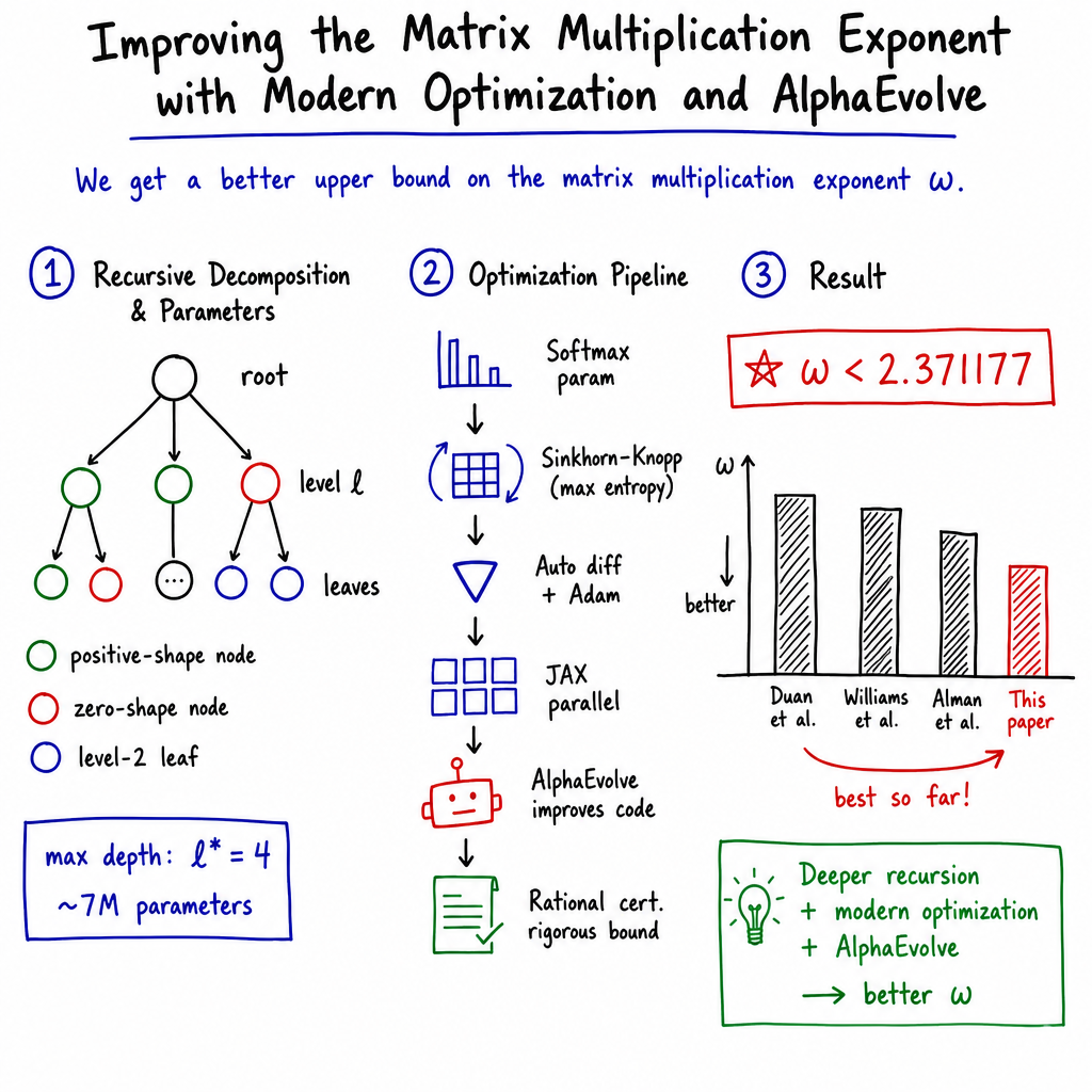
These choices were represented using a large tree:
- The root represented the original large problem.
- Each branch represented a way to split the problem into smaller problems.
- The leaves represented the smallest pieces.
- Each point in the tree had numbers describing how likely or useful different choices were.
The researchers then searched for values of these numbers that would produce the smallest possible value of , an upper bound on .
Using probabilities and entropy
Many of the choices in the tree were represented as probability distributions. A probability distribution is simply a list of chances that add up to 1.
The calculations also used entropy, a measure of uncertainty or variety. For example, if a spinner has many equally likely outcomes, its entropy is high. If one outcome is almost certain, its entropy is low.
Entropy helped the researchers measure how many useful combinations remained after the problem was split.
Gradient-based optimization
The optimization problem was extremely complicated and had millions of adjustable values. For the larger version, the researchers used nearly 7 million parameters.
They used a method called gradient descent. A simple analogy is walking down a foggy mountain:
- The program measures which direction goes downhill.
- It takes a small step in that direction.
- It repeats this many times.
The aim is to reach a low point, where the value of is small.
The researchers used several modern machine-learning tools:
- Softmax, which converts unrestricted numbers into valid probabilities.
- Automatic differentiation, which automatically calculates how changing each parameter affects the result.
- Adam, an algorithm that adjusts parameters efficiently.
- Sinkhorn–Knopp, a method used to find probability distributions with particular totals or “margins.”
- JAX, software that allows many calculations to run in parallel on GPUs.
Improving the program with AlphaEvolve
After creating their optimization program, the researchers used AlphaEvolve to modify and improve the program itself.
AlphaEvolve tested different versions of the code. Versions that found better bounds were kept and used as starting points for further improvements. This is somewhat like natural selection: better-performing versions survive and produce new versions.
Rigorous checking
Computer searches normally use decimal approximations, which can contain tiny errors. Since this work is part of a mathematical proof, the researchers performed a separate verification step.
They:
- converted the computer’s results into exact fractions,
- used rational arithmetic instead of ordinary floating-point arithmetic,
- carefully rounded logarithms in safe directions, and
- checked that every required inequality still held.
This was intended to ensure that the claimed bound was a valid proof, not merely a promising numerical result.
4. What did they find?
The main result was:
This improves the previous best result of $2.371339$.
| Result | Upper bound for |
|---|---|
| Earlier result | $2.371339$ |
| This paper | $2.371177$ |
The improvement is small in size, but it is meaningful because progress on this problem has been very difficult. The researchers achieved it in two main stages:
- Gradient-based optimization improved the previous result.
- AlphaEvolve further improved the optimization program and produced the final bound.
The new approach also allowed the researchers to study a deeper recursion level, , instead of stopping at . In simple terms, they could analyze one more layer of problem-splitting, although this made the number of parameters grow from roughly 25,000 to about 7 million.
5. Why is this important?
The result improves our theoretical understanding of how efficient matrix multiplication can be. Since matrix multiplication appears inside many important algorithms, faster methods could eventually help with:
- training and running AI systems,
- processing large datasets,
- computer simulations,
- computer graphics, and
- other scientific calculations.
However, the paper does not immediately make ordinary matrix multiplication programs faster. The improvement concerns an asymptotic bound, which describes what happens for extremely large matrices. Practical programs may still use other methods because they are simpler or faster for the matrix sizes commonly used today.
Conclusion: What could this lead to?
This paper shows that modern machine-learning ideas and AI-assisted programming can help solve difficult mathematical optimization problems. The researchers used AI not to replace the proof, but to search for promising numerical settings and better algorithms. They then checked the result with exact mathematics.
The work suggests that AI may be useful as a partner in mathematical research, especially when a problem involves millions of possible choices. At the same time, the authors point out that larger improvements will probably require new mathematical ideas, not only better optimization.
In short, the paper makes a small but genuine step toward understanding the fastest possible way to multiply matrices, while also demonstrating how computers and AI can assist in creating and checking advanced mathematical proofs.
Knowledge Gaps
Knowledge gaps, limitations, and open questions
- The paper does not provide the complete optimized parameter vector, executable implementation, or verification repository; independent reproduction of the certified bound is therefore not currently possible.
- The reported improvement is not accompanied by a detailed ablation study separating the effects of gradient descent, JAX/tensor parallelization, Sinkhorn optimization, implicit differentiation, and AlphaEvolve.
- The contribution of AlphaEvolve is not quantified across multiple independent runs, random seeds, population sizes, generations, or computational budgets, leaving the robustness and reproducibility of its improvement unclear.
- The paper does not report optimization failure rates, variance across runs, convergence curves, or the number of candidate solutions evaluated before obtaining the bound .
- It is unclear whether the final result is close to the best solution within the specified , optimization formulation, since no optimality certificate, lower bound on the optimization objective, or systematic comparison with alternative optimizers is provided.
- The optimization is performed only for and ; the relative performance of other values of and recursion depth is not investigated.
- The paper does not determine whether increasing beyond $4$ yields meaningful improvements or whether the computational and memory costs become prohibitive.
- The interaction between the hyperparameters and is left unexplored, including whether joint tuning could produce a stronger bound than the reported fixed choice.
- The computational cost of the complete procedure is incompletely characterized: training time, total GPU hours, memory usage, hardware configuration, and AlphaEvolve’s aggregate resource consumption are not reported in sufficient detail.
- The numerical optimization uses softmax logits, but the effects of probability underflow, saturation, near-zero masses, and ill-conditioning on the resulting solution are not analyzed.
- The stability and accuracy of differentiating through Sinkhorn iterations are not empirically validated against exact or independently computed maximum-entropy solutions on representative instances.
- The paper does not specify the Sinkhorn stopping criteria, regularization choices, iteration counts, initialization, or convergence diagnostics needed to reproduce the gradients and objective values.
- The maximum-entropy certification procedure is described abstractly, but the construction of the certificate distributions, Lagrange multipliers, and residual bounds for the final solution is not disclosed.
- The universal additive error bound in the maximum-entropy lemma may be loose; the paper does not assess how much this certification slack contributes to the final value of .
- The effects of rational rounding and directed logarithm approximations on the final certified bound are not quantified, so the gap between the unrounded numerical objective and the rigorous value remains unknown.
- The paper does not provide the exact certified value of before rounding, the rational precision used, or the size and structure of the resulting certificate.
- The claim that the final bound is rigorous depends on a verification implementation that is still being prepared; until released and independently audited, software or transcription errors cannot be ruled out.
- The manuscript contains apparent LaTeX, notation, and formatting corruption in several definitions and equations, making it difficult to determine the exact optimization problem and weakening the verifiability of the formal presentation.
- The paper relies on the theorem from prior work that any feasible solution implies an upper bound on , but does not independently re-derive how the altered implementation and expanded parameterization satisfy all assumptions of that theorem.
- It is not established whether the tensor decomposition represented by the enlarged tree and parameterization is genuinely more expressive than the formulation, or whether the improvement arises primarily from numerical search.
- The method remains confined to the Coppersmith–Winograd tensor and the combination-loss framework; it does not investigate whether the optimization and AlphaEvolve strategy applies to other tensors, laser-method variants, or fundamentally different matrix-multiplication constructions.
- The paper does not identify structural properties of the discovered solution that could lead to human-understandable mathematical improvements rather than further black-box numerical gains.
- The claim that larger improvements likely require new mathematical ideas is not supported by a systematic analysis of the current framework’s theoretical bottlenecks or an upper limit on improvements achievable within the chosen parameterization.
- No comparison is made with other modern global-optimization methods, such as evolutionary strategies, Bayesian optimization, population-based training, augmented Lagrangian methods, or mixed first-/second-order procedures.
- The effect of the phantom-node representation and masking is not separately evaluated, including whether the approximately threefold parameter increase harms optimization quality or introduces redundant degrees of freedom.
- The paper does not examine whether symmetries among coordinate permutations, shapes, and regions can reduce the seven-million-parameter search space without sacrificing the best achievable bound.
- The practical matrix-multiplication algorithm corresponding to the certified exponent is not constructed or evaluated; consequently, the work establishes an asymptotic upper bound but gives no information about finite-size constants, implementation complexity, or crossover points.
- The bound is asymptotic, and the paper leaves unresolved how large matrices must be before the associated construction becomes competitive with existing practical algorithms.
- The broader reproducibility and generalization of program-search-based mathematical optimization are not assessed beyond this single optimization task.
Practical Applications
Immediate Applications
- Research infrastructure for automated mathematical optimization — Academia / software engineering
- Potential tools: JAX-based optimization templates, differentiable combinatorial-search libraries, GPU-parallel solvers, and program-evolution pipelines.
- Dependency: The target problem must admit a differentiable or approximately differentiable formulation and have an objective that can be evaluated efficiently in parallel.
- Computer-assisted theorem proving and certification workflows — Academia / formal methods
- Potential workflow: neural or evolutionary search → candidate extraction → rationalization → interval/rational verification → publishable certificate.
- Dependency: The mathematical result must have a finite certificate and computable error bounds. Numerical optimization alone is not sufficient for a rigorous theorem.
- Benchmark for AI-assisted mathematical discovery — AI research / education
- Possible evaluation metrics: best certified bound, time-to-best-bound, GPU cost, robustness across random seeds, and certificate-generation success rate.
- Dependency: The released implementation, exact problem specification, and discovered parameter solutions must be publicly available and independently reproducible.
- Training and teaching material for computational complexity and scientific machine learning — Academia / education
- Potential product: graduate-level assignments or notebooks that reproduce smaller cases such as or .
- Dependency: Full-size reproduction is computationally demanding; educational versions would need reduced problem sizes and simplified certification code.
- Improved implementation strategies for structured GPU workloads — Software / high-performance computing
- Potential tools: compiler transformations or runtime libraries that convert irregular graphs into padded tensor representations.
- Dependency: Padding overhead, memory consumption, and masking costs must remain lower than the cost of conventional graph traversal.
- Methodological guidance for entropy-constrained optimization — Machine learning / optimization
- Dependency: Sinkhorn iterations may become numerically unstable or slow for ill-conditioned marginals, large supports, or highly sparse distributions.
- Long-horizon planning for hardware and algorithm libraries — Industry / computing
- Dependency: The bound concerns asymptotic arithmetic complexity and does not establish lower wall-clock time for practical matrix sizes, finite precision, memory movement, or hardware-specific architectures.
Long-Term Applications
- Asymptotically faster matrix multiplication libraries — Software, AI, graphics, and scientific computing
- Required development: Extract explicit multiplication schemes from the combination-loss construction, optimize constants, support finite matrix dimensions and numerical stability, and compare against highly tuned classical and Strassen-like methods.
- Key assumption: The asymptotic improvement must survive the substantial overheads of recursion, data movement, temporary storage, and numerical error.
- Lower-cost large-scale machine-learning systems — AI infrastructure
- Potential products: compiler-selected multiplication algorithms, accelerator kernels, and hardware architectures specialized for non-classical recursive schemes.
- Dependencies: The method must work efficiently with low-precision arithmetic, tolerate rounding error, map well to distributed accelerators, and avoid communication overhead that overwhelms the arithmetic savings.
- Energy-efficient scientific and engineering simulation — Energy, climate modeling, physics, and engineering
- Potential workflow: numerical software detects suitable matrix dimensions and sparsity patterns, then selects a certified fast multiplication kernel.
- Dependency: Most real-world simulation matrices are sparse, structured, rectangular, or ill-conditioned; the paper’s result primarily concerns asymptotic multiplication of dense matrices and may not transfer directly.
- Specialized hardware accelerators — Semiconductors / robotics / edge computing
- Required research: hardware–algorithm co-design, memory-layout optimization, fault tolerance, low-precision variants, and efficient handling of irregular recursion.
- Dependency: Hardware deployment requires stable, regular, and sufficiently low-overhead computation; the current optimization representation uses masking and may incur hardware inefficiency.
- General-purpose AI systems for mathematical algorithm discovery — AI research / industry R&D
- Potential product: a “proof-producing algorithm discovery” platform that proposes code and returns independently checkable certificates.
- Dependencies: Search systems must avoid reward hacking, preserve mathematical validity, provide interpretable outputs, and operate under strong reproducibility and security controls.
- Automated discovery of improved algorithms for other algebraic operations — Theoretical computer science / cryptography / symbolic computation
- Required research: formulate suitable finite optimization problems, identify certifiable relaxations, and establish theorems connecting feasible solutions to algorithmic upper bounds.
- Dependency: Matrix multiplication has unusually rich algebraic structure; comparable reductions may not exist for other problems.
- Policy and funding priorities for reproducible AI-assisted science — Research policy
- Potential policy instruments: certificate requirements, reproducibility checklists, archival standards for evolved programs, and independent verification grants.
- Dependency: Verification standards must be practical across disciplines and should address proprietary software, nondeterministic hardware, and the environmental cost of extensive search.
- Everyday applications through downstream computational savings — Daily life / consumer technology
- Dependency: These benefits require successful commercialization, hardware integration, and measurable reductions in total system cost—not merely a small improvement in the asymptotic exponent.
- Important feasibility limitation across all downstream uses — Cross-sector The reported result is an improvement in the theoretical upper bound, from approximately $2.371339$ to $2.371177$, rather than a demonstrated production algorithm or benchmarked speedup. The practical impact therefore depends on several unresolved factors: explicit algorithm extraction, constants, finite-size crossover points, memory traffic, parallel communication, numerical stability, software engineering, and independent reproduction of the certificate. Until these are addressed, the most credible applications are in research tooling, optimization methodology, automated discovery, and formal verification, rather than immediate replacement of existing matrix-multiplication libraries.
Glossary
- Adam: An adaptive gradient-based optimization algorithm that adjusts learning rates for individual parameters. “We update the parameters using Adam \citep{kingma2015adam}.”
- asymptotic matrix multiplication exponent: The limiting exponent governing the number of operations required to multiply increasingly large matrices. “where is the asymptotic matrix multiplication exponent.”
- automatic differentiation: A method for computing derivatives of programs by systematically applying the chain rule. “We compute the gradients of the objective using automatic differentiation.”
- Cartesian product: The set of ordered combinations formed by selecting one element from each of two or more sets. “where denotes the Cartesian product of complete split distributions”
- certificate residual: A bounded discrepancy used to verify that a proposed distribution satisfies the conditions needed for an entropy bound. “a real number satisfying, for every ”
- combination loss analysis: A refinement of the laser method that analyzes losses arising when multiple recursive decompositions are combined. “The current best bound is achieved by a refinement of the laser method called combination loss analysis”
- complete split distribution: A probability distribution over vectors whose entries encode how a coordinate is divided across recursive tensor factors. “A distribution over is called a level- {complete split distribution} of .”
- concave: Having the property that a function lies above the line segment joining any two points in its domain. “The entropy function is concave on ”
- constraint qualification: A technical condition ensuring that constrained optimization problems have well-behaved solutions or multipliers. “the problem constraints.”
- Coppersmith–Winograd tensor: A structured tensor used in fast matrix multiplication constructions and analyses. “where is the Coppersmith-Winograd tensor”
- differentiable objective: An objective function whose derivatives exist and can therefore be used by gradient-based optimization. “To apply a gradient-based optimization algorithm, we need a differentiable objective function to be optimized.”
- double exponential: Growth proportional to an exponential applied to an exponential, such as . “the complexity of the optimization (which grows doubly exponentially in )”
- entropy: A measure of uncertainty in a probability distribution, calculated here using base-two logarithms. “For a distribution with finite support, we denote its entropy by”
- feasible solution: An assignment of variables satisfying every constraint in an optimization problem. “Any feasible solution of \Cref{eq:optimization-problem} implies ”
- floating-point error: Numerical inaccuracy caused by representing real numbers with finite-precision binary formats. “to guard against floating point errors.”
- gradient descent: An optimization method that iteratively updates parameters in the direction that decreases an objective function. “we leverage recent advances in machine learning and adjacent areas to address the non-convex optimization problem”
- hardware parallelization: The simultaneous execution of computations across multiple hardware processing units. “allows for hardware parallelization”
- implicit differentiation: Differentiation through variables defined implicitly by equations or optimization conditions rather than by explicit formulas. “we employ implicit differentiation for backpropagating through the Sinkhorn-Knopp algorithm”
- Lagrange multiplier: An auxiliary variable used to represent constraints when optimizing a function subject to equality or inequality conditions. “these values play the role of Lagrange multipliers for the maximization defining ”
- laser method: A technique for extracting matrix multiplication algorithms from recursively structured tensors. “All improvements in the past 40 years rely on the laser method”
- logit: An unconstrained real-valued parameter that is transformed into a probability, typically using softmax. “we parameterize distributions in terms of their logits”
- marginal distribution: The distribution of one coordinate obtained by summing over all other coordinates. “let denote the marginal of in coordinate ”
- mass: A scalar weight assigned to a node that represents its contribution within the recursive decomposition. “Each non-zero-shape node of the tree has a real number associated with it, called its {mass}.”
- non-convex optimization: Optimization in which the objective or feasible region is not convex, so local optima may not be globally optimal. “a non-convex optimization problem as part of the computer-assisted proof”
- optimal transport: The study of efficiently transforming one probability distribution into another while minimizing a transport cost. “We develop an algorithm applying several techniques from machine learning and adjacent areas, such as optimal transport.”
- penalty: The difference between a constrained maximum entropy and the entropy of a given distribution. “as well as the penalty notion”
- positive-shape node: A tree node whose three shape coordinates are all strictly positive. “We call a non-root node a {positive-shape node} if all coordinates in its shape are positive.”
- rational arithmetic: Exact computation using rational numbers rather than finite-precision approximations. “we run a separate verification step computing all quantities in rational arithmetic”
- retained exponent: An exponent measuring the contribution preserved by the recursive tensor decomposition. “Next, we define how to calculate the {retained exponent} associated with the root ”
- rooted tree: A tree graph with one designated node called the root. “The high-level structure of the optimization problem can be captured by a rooted tree”
- sequential quadratic programming (SQP): A constrained optimization method that repeatedly solves quadratic programming approximations to a nonlinear problem. “this was done (for ) via a sequential quadratic programming (SQP) algorithm”
- shape: A triple of nonnegative integers describing the allocation among the three tensor dimensions. “A level- {shape} is a triple ”
- simplex: The set of nonnegative vectors whose entries sum to one, representing probability distributions. “For any finite set , we use to denote the simplex of probability distributions on ”
- Sinkhorn–Knopp algorithm: An iterative matrix-scaling algorithm used to find distributions with prescribed marginals. “the Sinkhorn-Knopp algorithm \citep{sinkhorn1967concerning} is used to obtain a stable and differentiable objective”
- softmax: A function that converts real-valued scores into nonnegative values summing to one. “we obtain the distribution by applying the softmax operation on the free parameters.”
- support: The subset of a distribution’s domain containing elements with nonzero probability. “where $\supp(\beta)$.”
- tensor decomposition: The representation of a tensor as a structured combination of simpler tensors. “the tree structure describes a recursive way to decompose the tensor”
- valid certificate: A collection of distributions and numerical parameters that proves an upper bound on a maximum entropy. “For a set of shapes and a probability distribution , a {valid certificate} for consists of:”
- zero-shape node: A tree node whose shape has at least one coordinate equal to zero. “Otherwise it is a {zero-shape node}.”

