The Hayman--Wu constant is
Abstract: We show that for every conformal map from the unit disk onto a simply connected proper domain , the length of is at most for every line .
Paper Prompts
Sign up for free to create and run prompts on this paper.
Top Community Prompts
Explain it Like I'm 14
1. What is the paper about?
This paper studies how long a straight line can appear inside a complicated shape after the shape has been transformed by a special kind of function called a conformal map.
A conformal map changes the shape of a region while preserving angles. Imagine drawing a picture on a rubber sheet and stretching or bending the sheet without making sharp corners. The paper asks:
If we start with the unit disk and reshape it using a conformal map, how much of a straight line can lie inside the new shape, when measured back in the original disk?
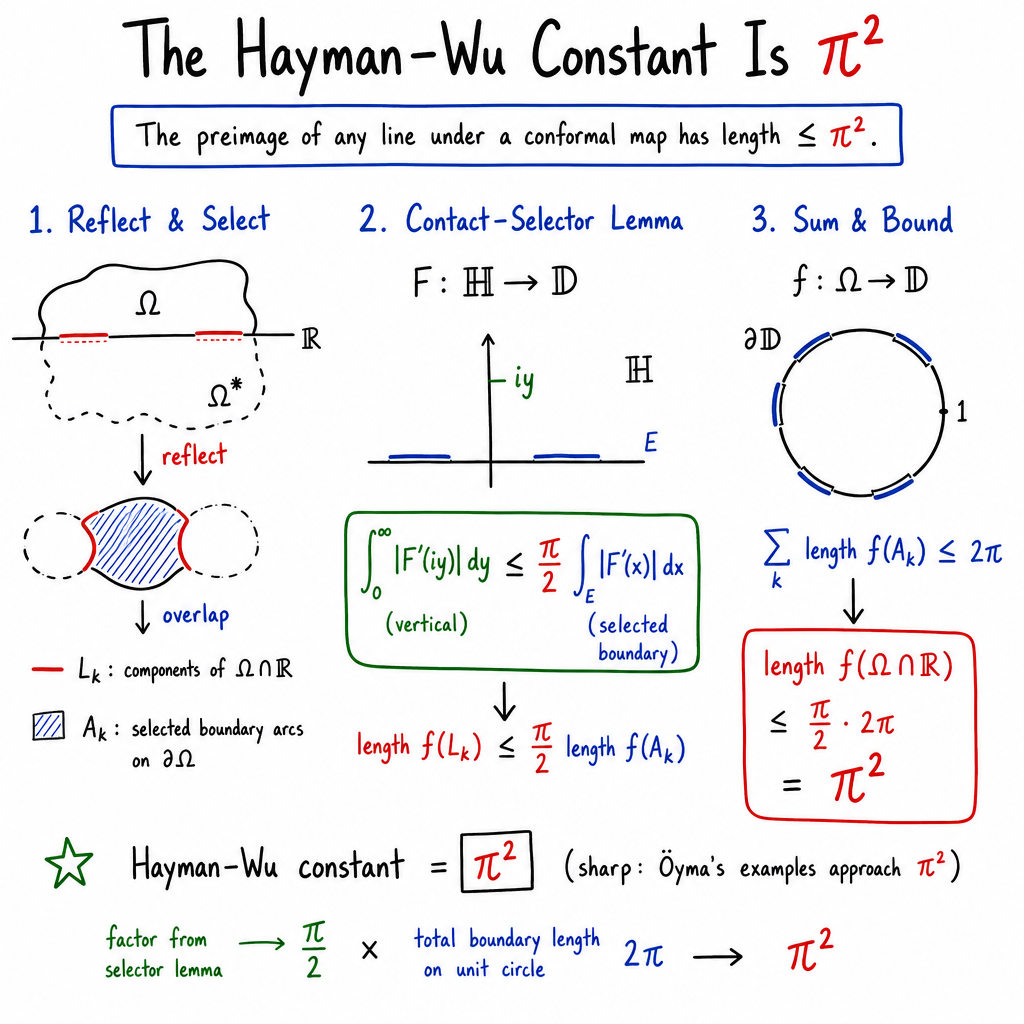
The paper proves that the answer is never more than
This number is the best possible answer. In other words, there are examples that get arbitrarily close to , but no example can go beyond it.
2. What questions does the research ask?
The main research question is:
For every conformal map from the unit disk to a simply connected region, and for every straight line, is the length of the part of that line inside the region always bounded?
Earlier mathematicians had proved that such a bound exists, but they did not know the exact smallest bound.
The paper aims to:
- Prove that the length is always at most .
- Show that is the exact best constant.
- Develop a new estimate, called the contact-selector lemma, that makes the sharp result possible.
Here, “sharp” means that the bound cannot be improved.
3. How did the researchers approach the problem?
Step 1: Simplifying the shape
The researchers first handle especially nice regions whose boundaries are smooth curves. These are called analytic Jordan domains.
They also rotate and move the picture so that the line being studied becomes the real axis.
To understand the region better, they reflect it across the real axis and compare the original region with its reflection. The overlapping pieces are divided into smaller regions.
This is similar to looking at an object and its mirror image to find the parts that match.
Step 2: Mapping the pieces back to the disk
Each overlapping piece is mapped from the upper half-plane to the piece using a conformal map. The upper half-plane is
The researchers then use the inverse of the original map to send these pieces back into the unit disk.
They compare two kinds of curves:
- the part lying on the real axis, which corresponds to the line inside the region;
- selected pieces of the boundary, which lie on the edge of the original region.
Step 3: The contact-selector lemma
The key new result is the contact-selector lemma.
In simple terms, it says:
The length of the image of the vertical half-line is at most times the length of certain selected boundary pieces.
The selected boundary pieces are chosen carefully: from every pair of mirror-image boundary intervals, the researchers choose the one that lies on the original boundary.
The factor comes from estimating how much a curve can be stretched when it moves from the boundary toward the inside. The proof uses several tools from complex analysis:
- Schwarz–Pick estimates, which control how much holomorphic maps can stretch;
- factorization, which separates a function into simpler parts;
- Herglotz representation, which describes certain functions using positive measures;
- Schwarz reflection, which extends a function across a smooth boundary as if the boundary were a mirror.
These are advanced mathematical tools, but their shared purpose is fairly simple: they prevent the map from stretching the inside too much compared with the boundary.
Step 4: Adding the pieces together
The selected boundary pieces from different regions do not overlap, except possibly at their endpoints. Therefore, their total length cannot exceed the circumference of the unit circle:
For each piece, the paper obtains an estimate of the form
Adding all the pieces gives
Step 5: Handling general regions
Finally, the researchers approximate an arbitrary simply connected region by nicer regions inside it. As these approximating regions grow toward the original one, their lengths approach the original length.
This is like estimating the area of an irregular shape by using increasingly accurate smaller shapes. The bound remains valid in the limit.
4. What are the main findings?
The main theorem says:
If is a conformal map from the unit disk onto any simply connected proper region , then for every straight line ,
The notation means that we look at the part of the line inside and map it back into the original unit disk.
The paper also uses earlier constructions showing that values can get arbitrarily close to . Therefore, the exact maximum is
This improves earlier bounds. For example, one earlier result gave the larger upper bound . The new result replaces that estimate with the smaller and exact value .
The important idea is that the paper does not merely prove that the length is finite. It finds the precise limit.
5. Why is this important?
This result helps mathematicians understand how conformal maps control length and shape.
Conformal maps are important in many areas, including:
- complex analysis;
- geometry;
- fluid flow;
- electrical problems;
- the study of shapes and boundaries.
The theorem shows that even though a conformal map can stretch and distort a region dramatically, it cannot make the preimage of a straight line arbitrarily long. There is a universal limit, and that limit is exactly .
The new contact-selector lemma is also useful because it provides a powerful way to compare interior curves with boundary curves. This method may help with other problems involving conformal maps, stretching, and the geometry of complicated regions.
In short, the paper solves the Hayman–Wu problem completely:
No conformal reshaping of the unit disk can make the relevant line length exceed , and this bound is the best possible.
Knowledge Gaps
Knowledge gaps, limitations, and open questions
- Equality cases are not characterized. The paper proves the sharp constant but does not determine whether equality is attained by any conformal map and line, or classify all possible extremizers if attainment occurs.
- The near-extremal geometry remains unspecified. Öyma’s examples show that lengths can approach , but the paper does not analyze the geometric structure of domains and maps that are nearly extremal or establish a quantitative stability theorem.
- The limiting behavior of Öyma’s examples is not investigated. It remains unclear whether extremizing sequences converge, after normalization, to a canonical degenerate domain or whether multiple geometrically distinct degeneration mechanisms exist.
- The approximation step is not quantified. The passage from an arbitrary simply connected proper domain to the domains proves the bound by monotone convergence, but does not provide error estimates in terms of , boundary regularity, or geometric data of .
- Boundary regularity beyond simple connectivity is not explored. The proof uses analytic Jordan domains as an intermediate class and then approximation, but does not determine whether analogous sharp estimates can be obtained directly for domains with rough, fractal, locally connected, or non-locally-connected boundaries.
- The role of boundary accessibility is left implicit. The argument relies on boundary parametrizations, Schwarz reflection, and disjoint boundary arcs in the analytic Jordan case; the corresponding interpretation of contact sets for general domains is not developed.
- Several planar separation facts are imported without proof. In particular, the assertions that the reflected components are Jordan domains and that distinct components have boundary intersections consisting of at most one point are cited as standard rather than established within the paper. Their precise hypotheses and applicability to all configurations are therefore not documented.
- The selector construction is not generalized to infinitely many boundary intersections. The analytic Jordan argument uses the fact that two analytic Jordan curves intersect finitely many times. The paper does not address how the selector argument would work when the reflected boundaries meet infinitely often or on sets of positive measure.
- The contact-selector lemma is proved only for finite unions of intervals. It is unknown whether the same inequality holds for arbitrary measurable selector sets satisfying the almost-everywhere choice condition, and what additional hypotheses would be needed for such an extension.
- Equality and near-equality conditions for the contact-selector lemma are not analyzed. Although the constant is shown to be sharp asymptotically using a Blaschke factor, the paper does not identify equality cases or quantify how close a function and selector must be to the extremal configuration.
- The factorization argument does not yield a structural classification. The decomposition separates a possible zero from a zero-free factor, but the consequences of simultaneous near-equality in the Blaschke and Herglotz estimates are not examined.
- The dependence on the line is not studied. The result treats every line uniformly, but the paper does not investigate how varies with the position and direction of , nor whether maximizers or near-maximizers of this quantity exist for a fixed .
- No analogous sharp result is given for other curves. The methods are tailored to reflection across a straight line; it remains open from this paper whether comparable universal bounds hold for circles, analytic arcs, quas lines, or more general rectifiable curves.
- The treatment is restricted to conformal maps from the disk in the plane. Extensions to multiply connected domains, other source surfaces, or quasiconformal maps are not addressed.
- The theorem concerns conformal length but not finer geometric quantities. The paper does not derive bounds for the number of components of , their distribution, endpoint behavior, or related harmonic-measure quantities.
- The relationship with previously studied reflected-component classes is not further clarified. The paper notes that Crane treated a broader class, but does not identify precisely whether the present contact-selector method yields new bounds or sharpness results for additional reflected-domain configurations.
- No quantitative dependence on normalization or domain geometry is provided. Apart from the universal constant, the result does not relate the conformal length to quantities such as diameter, inradius, quasidisk constants, smoothness norms, or harmonic measure of the intersected line.
Practical Applications
The paper proves a sharp geometric bound: for any conformal map onto a simply connected proper planar domain and any Euclidean line , the preimage of the line segment inside the domain has conformal arclength at most . The result is primarily foundational rather than directly technological; its practical value lies in providing certified geometric bounds, analysis tools, and design principles for conformal mappings, planar domains, and related numerical methods.
Immediate Applications
- Certified bounds for conformal-mapping software — computational geometry and software
- Numerical implementations of the Riemann mapping theorem can use as a universal validation bound for the computed quantity
1
length(phi^{-1}(Omega ∩ L)).- Given a discretized simply connected domain and a computed conformal map, software can flag numerical errors when the estimated conformal length substantially exceeds .
- This is applicable to mesh generation, shape analysis, image warping, and planar computational-geometry libraries.
- Dependencies: The numerical domain must be approximately simply connected, the map must be sufficiently accurate, and discretization and boundary-tracing errors must be controlled. The theorem gives an upper bound, not a direct numerical algorithm.
- Benchmarking conformal distortion in planar shape analysis — computer vision and graphics
- Conformal maps are used to flatten or normalize planar shapes. The theorem supplies a worst-case bound on how much a straight feature in the target plane can correspond to a curve in the parameter disk.
- It can therefore serve as a benchmark when comparing conformal parameterization methods for:
- texture mapping,
- planar object registration,
- document and handwriting normalization,
- shape matching,
- geometric image processing.
- Dependencies: The relevant feature must be representable as the intersection of the domain with a straight line after normalization. The bound concerns conformal preimage length, not ordinary Euclidean length in the original domain.
- Quality-control criterion for conformal flattening and mesh parameterization — CAD and graphics
- A workflow can combine a conformal map with line-sweep tests: sample lines in the flattened domain and estimate the lengths of their preimages.
- Values approaching identify geometries or boundary configurations with near-extremal conformal distortion and may indicate difficult regions for mesh generation or interpolation.
- Dependencies: Near-extremal behavior may be sensitive to boundary resolution. The theorem applies to simply connected proper domains; holes or multiply connected geometries require different results.
- Improved theoretical guarantees for harmonic-measure and level-set computations — numerical analysis
- The proof connects conformal length with reflected domains, Schwarz reflection, boundary arclength, and Herglotz representations. These ingredients can guide error estimates for algorithms that compute:
- harmonic measure,
- level sets of univalent functions,
- boundary correspondence under conformal maps,
- trajectories and cross-sections in planar potential problems.
- The sharp constant replaces earlier general upper bounds such as , giving tighter worst-case guarantees in analyses that reduce to Hayman–Wu-type quantities.
- Dependencies: Translating the theorem into a numerical error bound requires additional assumptions about approximation schemes, smoothness, and stability.
- Adversarial and stress testing of planar conformal algorithms — software engineering
- The extremal examples associated with can be used to construct difficult test cases for conformal-map solvers.
- Testing against domains whose line-preimage lengths approach the sharp constant can reveal:
- loss of boundary accuracy,
- instability near narrow or nearly tangent regions,
- failure of reflection-based numerical routines,
- inaccurate treatment of unbounded or highly elongated geometries.
- Dependencies: The published theorem establishes sharpness through prior constructions, but a practical benchmark suite would require explicit numerical parametrizations of those examples.
- Reference theorem for mathematical education and research training — academia
- The result provides a compact example of how several classical tools combine to produce a sharp global estimate:
- conformal mapping,
- Schwarz reflection,
- factorization into Blaschke and zero-free components,
- Herglotz representation,
- boundary arclength formulas,
- approximation by analytic Jordan domains.
- It can be used in advanced courses and reading seminars in complex analysis, geometric function theory, and harmonic analysis.
- Dependencies: This is an educational and methodological application rather than a direct engineering deployment.
Long-Term Applications
- Adaptive conformal meshing with provable line-crossing limits — computational geometry and finite-element methods
- A future meshing system could use the theorem to constrain how complicated the preimage of a family of straight cuts can become under conformal parameterization.
- Possible workflow:
- 1. compute a conformal parameterization;
- 2. sweep target-plane lines through the parameter domain;
- 3. identify regions where preimage lengths approach the theoretical limit;
- 4. refine the mesh or change the parameterization locally.
- This could improve robustness in simulations involving planar domains, such as electrostatics, fluid flow, or fracture geometries.
- Dependencies: A useful local refinement rule would require extensions from a global supremum bound to quantitative local or probabilistic estimates.
- Shape-complexity metrics based on sharp conformal length — computer vision and geometric modeling
- The quantity
1
sup_L length(phi^{-1}(Omega ∩ L))- could become a conformally normalized descriptor of planar shape complexity.
- Shapes with values close to would be classified as difficult or highly distorted under line-based probing, while lower values could indicate more regular geometries.
- Potential uses include shape retrieval, anomaly detection, and selecting parameterization methods.
- Dependencies: The quantity depends on the chosen conformal map, which is generally not unique without normalization. A practical descriptor would need a canonical normalization and stable estimators under noisy boundaries.
- Design of conformal optical and microfluidic structures — photonics and fluid engineering
- Conformal transformations are used to design planar optical devices and solve two-dimensional potential-flow or diffusion problems. The theorem could provide a universal constraint on the complexity of transformed straight interfaces or measurement paths.
- In principle, it could help bound the conformal length of sensor lines, channel cross-sections, or optical rays after mapping a complicated device geometry to a reference domain.
- Dependencies: Physical interpretation requires a model in which the relevant observable is conformal length. Three-dimensional effects, material inhomogeneity, nonconformal transformations, and multiply connected domains are outside the theorem’s direct scope.
- Extension to multiply connected or rough domains — mathematical research with downstream applications
- Many practical geometries contain holes, cracks, islands, or rough boundaries. Extending the sharp bound to multiply connected domains, quasidisks, or less regular boundaries could make it more useful in engineering and data-driven geometry.
- Research directions include:
- bounds depending on connectivity,
- versions for quasiconformal maps,
- estimates for rectifiable or fractal boundaries,
- stability under domain perturbations,
- quantitative near-extremizer classification.
- Dependencies: The current proof relies substantially on simple connectivity, analytic or Jordan-domain approximation, reflected components, and boundary homeomorphisms.
- Automated theorem-aware verification of conformal solvers — formal methods and scientific computing
- The theorem’s decomposition into a contact-selector estimate and a global boundary-length estimate could inspire certified computational pipelines.
- A future solver might verify:
- approximate univalence,
- selector-side boundary correspondence,
- disjointness of reflected boundary arcs,
- numerical estimates below the threshold.
- Such a system could provide mathematically certified output for high-precision conformal mapping.
- Dependencies: Certification would require rigorous interval arithmetic or validated complex analysis, together with computable representations of domains and boundary curves.
- Generalization to other level sets and geometric probes — analysis and applied potential theory
- The paper concerns intersections with straight lines. Related bounds for circles, curves, equipotential lines, or families of analytic arcs could yield tools for:
- potential-flow analysis,
- level-set tracking,
- geometric optics,
- planar robotics and path planning,
- boundary-based sampling.
- The contact-selector method may provide a template for converting interior length estimates into selected boundary-length estimates.
- Dependencies: Straight lines are especially compatible with reflection symmetry and the half-plane model. Other probes may require new reflection principles, selector constructions, or curvature-dependent constants.
- Robotic and geometric path-planning heuristics in conformally parameterized environments — robotics
- In environments represented by simply connected planar domains, conformal maps can transform complicated workspaces into simpler reference domains. The theorem could eventually bound the conformal complexity of paths generated by line sweeps in the reference coordinates.
- This may support guaranteed exploration or coverage algorithms in planar environments.
- Dependencies: The theorem does not bound shortest-path length, physical travel distance, collision risk, or time. A robotics application would require additional metric comparisons and treatment of obstacles, which generally make the domain multiply connected.
- Policy and standards for reproducible conformal geometry computations — scientific governance
- The sharp universal constant can serve as a reference requirement in benchmarks and validation protocols for software used in conformal mapping and planar geometric analysis.
- Standards could require reported computations to include:
- domain connectivity assumptions,
- map normalization,
- boundary regularity,
- estimated conformal line lengths,
- numerical error bounds,
- comparison with the ceiling.
- Dependencies: Such standards would be relevant only to specialized scientific and engineering software; the theorem does not itself establish regulatory thresholds for physical systems.
Glossary
- Analytic Jordan domain: A domain whose boundary is a Jordan curve that is analytic, meaning locally representable by a convergent power series. “assume that is an analytic Jordan domain”
- Borel set: A set generated from open sets through countable unions, countable intersections, and complements. “these Borel sets increase to ”
- Carathéodory theorem: A theorem stating that a conformal map of a Jordan domain onto the unit disk extends continuously and homeomorphically to the boundary. “By symmetry and the Carathéodory theorem”
- Conformal length: The Euclidean arclength measured after applying a conformal map or its inverse. “Key words and phrases. Hayman--Wu theorem, conformal length”
- Conformal mapping: An angle-preserving holomorphic bijection between planar domains. “there is a conformal map”
- Contact-selector estimate: An inequality that bounds the length of an image on an interior line by the length of a suitably selected boundary subset. “The new input is the contact-selector estimate”
- Extended sense: The convention of allowing a nonnegative integral to take the value infinity before proving it is finite. “All nonnegative integrals below are understood in the extended sense until finiteness has been established.”
- Herglotz representation: An integral representation of holomorphic functions with nonnegative imaginary part in terms of a positive measure. “The Herglotz representation \cite[Chapter~I]{Duren} has the form”
- Holomorphic continuation: Extension of a holomorphic function beyond its original domain. “holomorphic continuation with real boundary values through an interval implies that has no mass there.”
- Inner approximation: Approximation of a domain or set from within by smaller domains or sets. “After an inner approximation and a Euclidean motion”
- Jordan curve: A simple closed curve in the plane, typically homeomorphic to a circle. “the two analytic Jordan curves and meet only finitely many times.”
- Jordan domain: A planar domain whose boundary is a Jordan curve. “The domain is a bounded analytic Jordan domain.”
- Lebesgue measure: The standard measure assigning lengths to subsets of the real line and areas to subsets of the plane. “The selector has infinite Lebesgue measure.”
- Möbius transformation: A fractional-linear map of the form , with . “”
- Nonvanishing function: A function that has no zeros on the domain under consideration. “On every interval contained in , the function extends holomorphically, is nonvanishing, and is unimodular.”
- Pick function: A holomorphic function mapping the upper half-plane into itself. “either is real constant or is a Pick function.”
- Schwarz reflection principle: A theorem allowing a holomorphic function with suitable real or symmetric boundary values to be extended across a boundary curve or interval. “the Schwarz reflection principle extends holomorphically across the interval.”
- Schwarz--Pick theorem: A fundamental inequality controlling holomorphic self-maps of the disk or upper half-plane in the hyperbolic metric. “Schwarz--Pick gives in the first case.”
- Simply connected domain: A domain in which every closed curve can be continuously contracted to a point. “for every conformal map from the unit disk onto a simply connected proper domain”
- Stieltjes inversion formula: A formula recovering a measure, or its density, from boundary values of an associated Cauchy or Stieltjes transform. “By the standard Stieltjes inversion formula”
- Tonelli’s theorem: A measure-theoretic result permitting the interchange of integration order for nonnegative measurable functions. “Hence, by Tonelli”
- Univalent function: An injective holomorphic function. “Let be univalent”
- Unimodular function: A complex-valued function whose absolute value is one. “ on .”
- Upper half-plane: The set of complex numbers with positive imaginary part. “Throughout, ”
- Weak boundary values: Values or limiting behavior of a function approached from within a domain at boundary points, often interpreted almost everywhere. “with real boundary values”
- Zero-free factor: A factor in a function factorization that has no zeros in the domain. “The zero-free factor.”

