A lower bound for stepsize-based acceleration of gradient descent

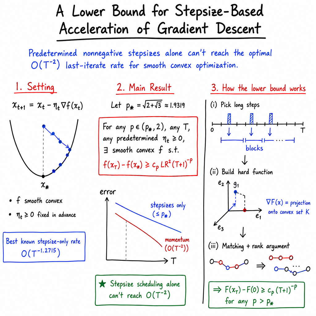
Abstract: Recent work has shown that, for smooth convex optimization, plain gradient descent can be accelerated from its textbook convergence rate of $O(T<sup>{-1})$ (where $T$ denotes the number of iterations) to $O\big(T<sup>{-\log_2(1+\sqrt{2})}\big)$ using carefully designed stepsize schedules alone, without resorting to momentum or other algorithmic modifications. Despite this progress, however, little was known about lower bounds for such methods beyond the classical $Ω(T<sup>{-2})$ benchmark for general first-order methods. In this work, we present a new lower bound of $Ω(T<sup>{-1.9319})$ for the last-iterate convergence rate of gradient descent with predetermined nonnegative stepsize schedules. This result provides rigorous evidence that stepsize schedules alone cannot accelerate plain GD to the optimal $O(T<sup>{-2})$ convergence rate. The proof was developed by GPT-5.6 Sol Pro under the authors' guidance.

• The paper proves that every predetermined nonnegative stepsize schedule has a smooth convex worst-case instance with terminal error at least c_p LR²(T+1)^(-p) for every p > √(2+√3) ≈ 1.9319, ruling out the optimal O(T^-2) rate.
• The authors reduce schedule analysis to a combinatorial functional over long steps, then combine an explicit Moreau-envelope hard instance with matching bounds and a Lyapunov argument to obtain the schedule-independent lower bound in dimension at most T+1.
• The result separates schedule-only gradient descent from general accelerated first-order methods, while leaving the exact achievable exponent between the best known 1.2715 upper bound and the 1.9319 lower-bound threshold unresolved.

Problem setting and principal result

The paper studies the worst-case last-iterate convergence of gradient descent on smooth convex objectives when the algorithm uses a predetermined, nonnegative stepsize schedule tailored to a prescribed horizon. The iteration is

$x_{t+1}=x_t-\eta_t\nabla f(x_t),$

where the schedule is fixed before the dimension, objective, and minimizer are selected. No restriction is imposed on the ordering or magnitude of the stepsizes: schedules may contain zero steps, arbitrarily large steps, and updates that increase the objective value. The analysis concerns only the terminal point $x_T$, not the best or averaged iterate.

For the standard choice $\eta_t=1/L$, gradient descent has a worst-case objective-gap rate of $O(LR^2/T)$. General first-order methods can attain the optimal $O(LR^2/T^2)$ rate, whereas recent work has shown that unmodified gradient descent can improve over $T^{-1}$ solely through horizon-dependent long-step schedules. In particular, silver-ratio schedules achieve an exponent

$\log_2(1+\sqrt{2})\approx 1.2715$

for suitable horizons and, through composition techniques, for arbitrary horizons. The central question is whether stepsize scheduling alone can reach the optimal exponent $2$.

The paper proves that it cannot, at least in the following quantitative sense. Let

$p_\star=\sqrt{2+\sqrt{3}}\approx 1.9319.$

For every $p\in(p_\star,2)$, every horizon $x_T$0, every $x_T$1, and every predetermined nonnegative schedule, there exists a dimension $x_T$2, a convex $x_T$3-smooth function $x_T$4, and an initial point at distance $x_T$5 from a minimizer such that

$x_T$6

where $x_T$7 depends only on $x_T$8. Equivalently, no such schedule can guarantee an $x_T$9 rate for any exponent $\eta_t=1/L$0. The result therefore rules out an $\eta_t=1/L$1 guarantee for plain gradient descent with predetermined nonnegative stepsizes.

The theorem is strictly nonendpoint: it does not establish the lower bound at $\eta_t=1/L$2. Thus, the proved impossibility threshold is $\eta_t=1/L$3 in the usual exponent sense, but the exact endpoint remains untreated. The gap between the best known upper exponent, approximately $\eta_t=1/L$4, and the lower-bound threshold, approximately $\eta_t=1/L$5, is substantial.

Reduction to a schedule functional

The proof first normalizes the problem by setting $\eta_t=1/L$6, reducing to $\eta_t=1/L$7. Each normalized step is decomposed into a capped component and an excess component:

$\eta_t=1/L$8

The analysis defines the base mass

$\eta_t=1/L$9

and lets $O(LR^2/T)$0 denote the number of long steps, namely steps satisfying $O(LR^2/T)$1. Since each capped contribution is at most one,

$O(LR^2/T)$2

This decomposition separates the ordinary stepsize mass from the acceleration mechanism attributed to long steps. The empty selection of long steps already yields a lower bound proportional to

$O(LR^2/T)$3

which is of order $O(LR^2/T)$4 when all steps are short. The difficult part is showing that introducing large excesses cannot reduce the worst-case terminal error too aggressively.

For any selected subset of long steps, ordered according to their occurrence in the schedule, the trajectory is partitioned into blocks. Each block has a scale $O(LR^2/T)$5, and each selected long step is associated with a transition factor $O(LR^2/T)$6. The resulting schedule functional is

$O(LR^2/T)$7

The geometric construction establishes that, for every schedule,

$O(LR^2/T)$8

for some convex $O(LR^2/T)$9-smooth function in dimension at most $O(LR^2/T^2)$0. Consequently, proving a schedule-independent lower bound on $O(LR^2/T^2)$1 is sufficient to prove the optimization lower bound.

This reduction is important because it converts an adversarial optimization problem into a combinatorial-analytic problem over the schedule. The temporal ordering of long steps remains present in individual chain values, but the objective function itself need not be analyzed through a general interpolation or semidefinite-programming relaxation.

Geometric realization of hard instances

The hard instance is constructed using the Moreau envelope of a support function. Given a compact convex set $O(LR^2/T^2)$2 containing the origin, define

$O(LR^2/T^2)$3

where $O(LR^2/T^2)$4 is the support function of $O(LR^2/T^2)$5. The key identity is

$O(LR^2/T^2)$6

with $O(LR^2/T^2)$7 denoting Euclidean projection onto $O(LR^2/T^2)$8. Thus, by designing $O(LR^2/T^2)$9, the authors can prescribe which gradient vector is active at each portion of the gradient-descent trajectory while retaining global convexity and $T^{-1}$0-smoothness.

For a chain of $T^{-1}$1 selected long steps, the construction introduces orthogonal anchors

$T^{-1}$2

with amplitudes satisfying $T^{-1}$3. The block gradients are chosen so that the trajectory moves along a fixed ray within each block and the selected long step lands exactly at the next orthogonal anchor:

$T^{-1}$4

The convex set $T^{-1}$5 is the convex hull of the origin and the block gradients. Projection comparisons show that the intended gradient $T^{-1}$6 remains the projection throughout block $T^{-1}$7, provided

$T^{-1}$8

At the terminal point, the objective gap is exactly

$T^{-1}$9

Taking $\log_2(1+\sqrt{2})\approx 1.2715$0 maximizes the gap within the construction and produces the functional $\log_2(1+\sqrt{2})\approx 1.2715$1. The construction uses $\log_2(1+\sqrt{2})\approx 1.2715$2 dimensions, so the final hard instance has dimension at most $\log_2(1+\sqrt{2})\approx 1.2715$3.

This realization is stronger than a merely existential resisting-oracle argument in one respect: it gives an explicit globally defined smooth convex objective. It also covers zero steps and arbitrarily large steps without requiring descent, bounded iterates, monotonic objective values, or stepsizes below the usual stability threshold.

Removing temporal order through matching bounds

The principal technical obstacle is that the chain product depends on the chronological order of the selected long steps. To eliminate that dependence, the proof ranks the positive excesses by magnitude:

$\log_2(1+\sqrt{2})\approx 1.2715$4

For a cutoff $\log_2(1+\sqrt{2})\approx 1.2715$5, the residual mass is

$\log_2(1+\sqrt{2})\approx 1.2715$6

The $\log_2(1+\sqrt{2})\approx 1.2715$7 largest excesses are restored to their original temporal order, and the reciprocal local factors are represented as edge weights on a path. The internal edge kernel is

$\log_2(1+\sqrt{2})\approx 1.2715$8

The path is split into odd and even edges, which form two matchings. Maximizing each matching independently removes the temporal ordering and yields

$\log_2(1+\sqrt{2})\approx 1.2715$9

where $2$0 is the product of two optimal matching values. This is the key order-independent inequality.

The matching weights depend on the normalized reciprocal excesses through

$2$1

together with an auxiliary terminal weight. Their total excess-dependent mass is governed by

$2$2

The proof then establishes that the geometric mean matching cost $2$3 is controlled by $2$4. As $2$5 grows, the relevant estimate approaches

$2$6

Thus, whenever $2$7 is sufficiently small, $2$8 and the matching lower bound gains an exponentially favorable factor through $2$9. This alternative is especially powerful because it converts diffuse reciprocal excess mass into a large adversarial objective gap.

Rank cutoff and the threshold exponent

The second alternative occurs when the matching cost is not small. Fix $p_\star=\sqrt{2+\sqrt{3}}\approx 1.9319.$0 and define

$p_\star=\sqrt{2+\sqrt{3}}\approx 1.9319.$1

For sufficiently large $p_\star=\sqrt{2+\sqrt{3}}\approx 1.9319.$2, the proof obtains the dichotomy

$p_\star=\sqrt{2+\sqrt{3}}\approx 1.9319.$3

for some $p_\star=\sqrt{2+\sqrt{3}}\approx 1.9319.$4. If $p_\star=\sqrt{2+\sqrt{3}}\approx 1.9319.$5, then necessarily

$p_\star=\sqrt{2+\sqrt{3}}\approx 1.9319.$6

The latter inequality constrains the growth of the residual mass $p_\star=\sqrt{2+\sqrt{3}}\approx 1.9319.$7. Define

$p_\star=\sqrt{2+\sqrt{3}}\approx 1.9319.$8

This quantity measures the relative increase in residual mass when the rank cutoff changes from $p_\star=\sqrt{2+\sqrt{3}}\approx 1.9319.$9 to $p\in(p_\star,2)$0, since

$p\in(p_\star,2)$1

The exact adjacent-rank recursion

$p\in(p_\star,2)$2

is then used to control the cumulative sequence $p\in(p_\star,2)$3. A Lyapunov potential of the form

$p\in(p_\star,2)$4

yields a one-step drift estimate. After telescoping, this gives

$p\in(p_\star,2)$5

along any interval on which the large-matching-cost alternative persists.

The interpretation is that if long steps do not generate a favorable matching configuration, their ranked magnitudes cannot grow rapidly enough to make the residual mass explode. The two mechanisms are therefore complementary:

• Small matching cost produces a direct chain lower bound through $p\in(p_\star,2)$6.
• Large matching cost restricts residual-mass growth through the Lyapunov argument.

A bounded-rank argument handles the transition between these regimes. Combining the alternatives gives

$p\in(p_\star,2)$7

Using $p\in(p_\star,2)$8 and $p\in(p_\star,2)$9 yields

$x_T$00

The threshold $x_T$01 arises from the compatibility condition required by the two parts of the proof. Specifically,

$x_T$02

must hold so that a threshold $x_T$03 can be selected. Substituting $x_T$04 gives

$x_T$05

At equality, the admissible interval for $x_T$06 collapses. This is not merely a technical numerical constant in the final theorem; it identifies the point at which the matching estimate and Lyapunov growth estimate cease to overlap under the present proof architecture.

Relation to existing acceleration and lower bounds

The result is distinct from the classical $x_T$07 lower bound for deterministic first-order methods. That oracle lower bound applies to a much broader class, including accelerated methods, and therefore cannot distinguish ordinary gradient descent from methods using momentum or other state transformations. The present theorem targets the narrower class of plain gradient descent with a fixed nonnegative schedule and proves a strictly stronger impossibility statement for that class.

It also differs from lower bounds for time-invariant stepsizes, which only show that constant-step gradient descent remains at the $x_T$08 exponent. The theorem permits arbitrary horizon-dependent schedules and therefore addresses the mechanism responsible for silver-step acceleration.

The distinction from anytime schedules is equally important. In the prescribed-horizon model, a new schedule may be designed for every $x_T$09. An anytime schedule must be fixed as an infinite sequence and must provide guarantees at every possible stopping time. Existing anytime upper and lower bounds therefore do not directly imply the theorem here. Conversely, the present lower bound does not establish an anytime limitation.

The paper’s comparison with known upper bounds leaves the central quantitative question unresolved:

$x_T$10

in the sense that the best construction achieves exponent approximately $x_T$11, while the lower bound rules out every exponent strictly larger than $x_T$12. The theorem proves that schedule-only acceleration cannot attain exponent $x_T$13, but it does not identify the optimal achievable exponent.

Limitations and open questions

The result applies only to deterministic, predetermined, nonnegative stepsizes and to the unmodified last iterate. It does not cover adaptive schedules depending on observed gradients, randomized schedules, signed stepsizes, averaging, extrapolated outputs, or other modifications of the gradient-descent update. It also does not establish a lower bound for the best iterate,

$x_T$14

because independently hard instances for different prefixes do not yield a single instance that is simultaneously hard for all prefixes.

The endpoint $x_T$15 remains open, as does the exact optimal exponent between $x_T$16 and $x_T$17. The proof’s endpoint failure is explicitly localized: the matching estimate requires a strict $x_T$18, while the Lyapunov parameter reaches the boundary precisely at $x_T$19. Whether a sharper matching inequality, a different potential, or a different hard-instance construction can reach the endpoint is not resolved.

The theorem is also stated for general smooth convex optimization rather than strongly convex optimization. Although long-step schedules accelerate gradient descent in strongly convex settings, an analogous lower bound for horizon-dependent nonnegative schedules is not supplied.

Finally, the manuscript discloses that the main proof was developed with GPT-5.6 Sol Pro under author supervision and subsequently formalized in Lean 4. This disclosure does not alter the mathematical statement, but it is relevant to the paper’s provenance: the proof’s reliability rests on the authors’ verification, revision, and formalization process rather than on the generative system alone.

Conclusion

The paper establishes that predetermined nonnegative stepsize schedules cannot accelerate plain gradient descent on smooth convex objectives to the optimal $x_T$20 last-iterate rate. For every $x_T$21, it constructs a dimension-$x_T$22 smooth convex hard instance producing an $x_T$23 terminal gap. The proof combines an explicit Moreau-envelope realization, order-independent matching bounds, and a rank-based Lyapunov argument. It provides a quantitative separation between schedule-only gradient descent and optimal first-order methods, while leaving the exact schedule-based exponent, the endpoint threshold, and several broader method classes unresolved.