Difference-in-differences with "bad controls"
Abstract: This paper considers difference-in-differences identification strategies when the parallel trends assumption holds after conditioning on covariates that may themselves be affected by the treatment (often referred to as "bad controls"). We show that common approaches such as simply dropping bad controls are often ill-advised and develop two alternative approaches that allow bad controls to function as genuine controls despite being affected by treatment. First, we derive explicit conditions that rationalize conditioning only on pre-treatment values of the bad control, leading naturally to the Callaway and Sant'Anna (2021) estimator with pre-treatment values as covariates. Second, under a covariate unconfoundedness condition, we develop imputation and double/debiased machine learning estimators that recover the average treatment effect on the treated. We extend these results to staggered treatment adoption, provide pre-tests for the identifying assumptions, and apply the methods to study the effects of job displacement on earnings.
Paper Prompts
Sign up for free to create and run prompts on this paper.
Top Community Prompts
Explain it Like I'm 14
1. What is the paper about?
This paper explains how researchers can measure the effects of a treatment or event when an important variable is changed by that treatment.
The researchers focus on a method called difference-in-differences. This method compares:
- how outcomes change over time for a treated group, and
- how outcomes change over time for a similar untreated group.
For example, researchers might compare the earnings of people who lose their jobs with the earnings of similar people who do not lose their jobs.
The difficult problem is that some useful comparison variables—such as a person’s occupation—may themselves change because of the treatment. The paper calls these variables “bad controls.”
2. What questions does the paper ask?
The paper mainly asks:
- Why can it be a problem to directly control for a variable that changes after treatment?
- Is simply removing that variable from the analysis a good solution?
- How can researchers still use information from a changing variable without creating misleading results?
- Can these new methods be used when different people receive treatment at different times?
- What happens when these methods are used to study how job displacement affects earnings?
The central idea is that researchers should not automatically include or exclude a changing variable. Instead, they should try to estimate what that variable would have been without the treatment.
3. How did the researchers study the problem?
Difference-in-differences
Imagine two groups of students:
- Group A joins a special study program.
- Group B does not join it.
Researchers measure both groups’ test scores before and after the program. They then compare the changes.
If Group A’s scores rise by 10 points and Group B’s scores rise by 4 points, the estimated effect of the program is:
This method depends on the parallel trends assumption. This means that, without the treatment, both groups would probably have changed in similar ways.
The problem with “bad controls”
Suppose researchers study the effect of job displacement on earnings and control for a worker’s occupation after displacement.
That can be misleading because job displacement may cause the worker to move into a different occupation. The occupation measured after displacement is therefore partly an effect of the treatment.
It is like trying to measure the effect of a storm on people’s health while controlling for whether their houses were damaged. The storm may have caused the house damage, so using the damage as an ordinary control can distort the comparison.
The paper studies two common strategies:
- Using the bad control directly: Include the post-treatment variable as if it had not been affected by treatment.
- Dropping the bad control: Remove it completely from the analysis.
The authors show that neither strategy is generally reliable when the variable is truly a bad control.
The researchers’ two new approaches
The paper develops two alternative methods.
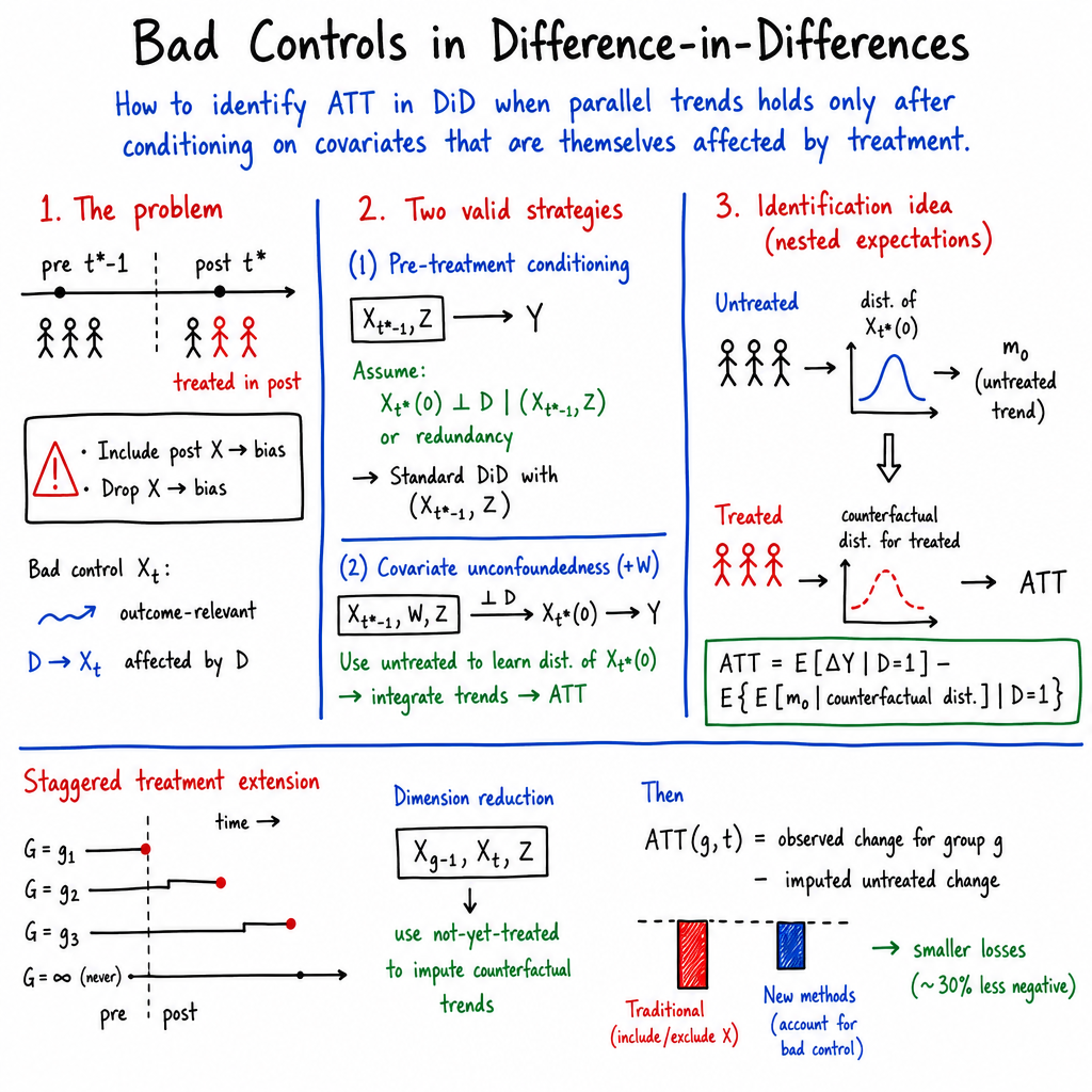
Approach 1: Use the pre-treatment value
The first method uses the variable’s value before treatment.
For example, when studying job displacement, researchers could compare people based on their occupation before displacement rather than their occupation afterward.
This approach assumes that people with the same pre-treatment characteristics would have had similar changes in the control variable if they had remained untreated.
In everyday terms, researchers use people who looked similar before the event to estimate what the treated people’s later situation would probably have looked like without the event.
Approach 2: Estimate the untreated version of the control
The second method is more flexible. It tries to estimate the value that the bad control would have had for treated people if they had not received treatment.
For example, researchers might use information about:
- a worker’s earlier occupation,
- earlier earnings,
- age, and
- other background characteristics.
They then look at untreated workers with similar characteristics to estimate the occupation the displaced workers would probably have had without displacement.
This is similar to reconstructing an alternate version of history: “What would this person’s occupation probably have been if the job loss had never happened?”
Technical tools
The paper proposes several statistical tools:
- Imputation: Fill in an unknown value using information from similar people.
- Doubly robust estimation: Use two different statistical models so that the estimate can still work if one model is wrong, as long as the other is reasonably correct.
- Double/debiased machine learning: Use computer algorithms to find complicated patterns in the data while reducing the risk that these patterns create bias in the final estimate.
These tools are not meant to replace careful reasoning. They help researchers handle large amounts of information and make more accurate predictions under the paper’s assumptions.
The authors also discuss ways to check whether the assumptions behind their methods seem reasonable. These checks are called pre-tests.
4. What did the paper find?
The paper reaches several important conclusions.
Directly including a bad control can create bias
If treatment changes the control variable, then using its post-treatment value does not represent the treated person’s untreated situation.
For example, if job displacement changes a worker’s occupation, controlling for the new occupation may produce an incorrect estimate of the effect of displacement on earnings.
Dropping the bad control can also be a mistake
Removing the variable does not automatically solve the problem.
If the variable really helps explain how outcomes would have changed without treatment, leaving it out may make the treated and untreated groups too different to compare fairly.
Therefore, dropping a bad control may simply replace one kind of bias with another.
The key missing information is a counterfactual
For treated people, researchers observe the control variable after treatment. But they do not observe what the variable would have been without treatment.
This missing value is called a counterfactual.
The paper’s methods try to estimate this counterfactual using untreated people with similar background characteristics.
The methods work in more complicated treatment settings
The researchers extend their methods to staggered treatment adoption, where different people receive treatment at different times.
This is useful because real-world policies and events rarely affect everyone at exactly the same moment.
Application to job displacement
The paper applies its methods to job displacement and earnings. It treats workers’ occupation scores as a bad control because job displacement can affect the occupations workers enter.
The researchers find that:
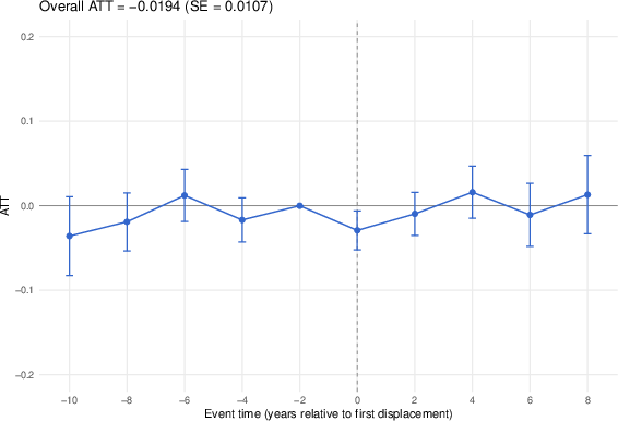
- job displacement lowers workers’ occupation scores on average;
- this supports the idea that occupation is affected by displacement and is therefore a bad control; and
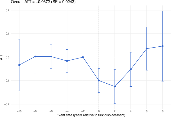
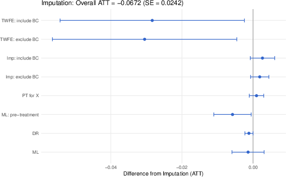
- the new methods estimate an effect of job displacement on earnings that is about 30% smaller than estimates from traditional methods that either directly include occupation or leave it out completely.
This shows that the choice of method can substantially change the conclusion of a study.
5. Why is this research important?
The paper warns researchers not to follow a simple rule such as “always include controls” or “always remove controls affected by treatment.”
Instead, researchers should ask:
- Was the variable measured before or after treatment?
- Could the treatment have changed it?
- Does the variable help explain how outcomes would have changed without treatment?
- Can the untreated version of the variable be estimated using similar untreated people?
The paper is especially important for economics, education, health, and social policy research, where treatments often change people’s jobs, locations, health conditions, or behavior.
Its main practical message is:
When a useful variable may be changed by treatment, researchers should estimate what that variable would have looked like without treatment rather than blindly using or discarding its observed value.
If these methods are used carefully, studies may produce more trustworthy estimates of the effects of policies and life events. However, the methods still depend on important assumptions and good-quality panel data—information about the same people measured at different times. If those assumptions are not believable, the true treatment effect may still be impossible to identify accurately.
Knowledge Gaps
Knowledge gaps, limitations, and open questions
- Identification depends on strong, largely untestable assumptions. The proposed estimators require conditional parallel trends and either simple or generalized covariate unconfoundedness, but the paper does not establish how credible these assumptions are in typical applications or how violations affect the ATT.
- The counterfactual distribution of the post-treatment covariate remains fundamentally assumption-dependent. For treated units, the distribution of cannot be observed, so the proposed methods recover it only under covariate unconfoundedness-type restrictions; the paper does not develop broadly applicable alternatives when these restrictions fail.
- The source and role of additional confounders are not fully characterized. The second approach assumes that the researcher observes all variables needed to make independent of treatment, but it does not provide a systematic strategy for discovering, measuring, or assessing the sufficiency of these variables.
- Sensitivity to unobserved confounding is not developed. The paper’s graphical discussion allows unobserved confounders in the general case, but it does not provide sensitivity analyses, partial-identification bounds, or quantitative bias formulas for violations of covariate unconfoundedness.
- The proposed pre-tests cannot generally verify the key counterfactual assumptions. Pre-tests based on observed pre-treatment data may detect some incompatibilities, but they cannot directly test conditional parallel trends involving for treated units or verify the absence of unobserved confounding.
- The relationship between the alternative identifying assumptions is not fully explored. Simple covariate unconfoundedness and bad-control redundancy are presented as non-nested routes to the same estimand, but the paper does not clarify when one is more plausible, how researchers should choose between them, or whether they can be combined to obtain testable implications.
- Finite-sample performance is insufficiently established in the provided text. The paper develops imputation, doubly robust, and double/debiased machine-learning estimators, but more evidence is needed on their finite-sample bias, variance, coverage, and stability under weak overlap, high dimensionality, and substantial treatment effects on the bad control.
- Weak or practically relevant overlap is not addressed in depth. The formal overlap conditions may be difficult to satisfy when the post-treatment covariate is continuous or high dimensional. The consequences of limited support, extreme propensity scores, trimming, and extrapolation are not fully analyzed.
- Inference with estimated counterfactual covariate distributions requires further clarification. The two-step and nested-estimation procedures may generate additional uncertainty and dependence beyond standard DiD estimators, yet the conditions and practical recommendations for valid standard errors, bootstrap procedures, and confidence intervals are not fully specified here.
- The methods are primarily developed for two-period designs and staggered adoption. Extensions to repeated treatments, treatment reversals, dynamic treatment regimes, event-study designs, and treatments with varying intensity are identified as possible future directions but are not developed.
- Treatment timing relative to covariate measurement is restrictive. The framework assumes that treatment occurs before the time-varying covariate and that the outcome is measured afterward. It does not fully address settings with multiple treatment and covariate measurements within a period, simultaneous determination, or uncertain treatment timing.
- Anticipatory effects are assumed away. No-anticipation is imposed for both the outcome and the bad control, but the paper does not develop diagnostics or estimators for settings in which treatment anticipation changes occupation, behavior, or outcomes before formal treatment.
- Interference and spillovers are excluded. SUTVA is imposed, leaving unresolved how the estimators behave when treatment affects other units’ covariates or outcomes, such as through labor-market competition, peer effects, or regional spillovers.
- Measurement error in bad controls is not considered. Misclassification or noisy measurement of occupation, industry, union status, or other time-varying covariates could distort both the estimated treatment effect on the covariate and the recovered counterfactual distribution.
- Attrition and sample selection are not addressed. The setup assumes an i.i.d. observed panel, but job displacement and similar treatments may affect employment, survey participation, or the probability of observing the bad control and outcome.
- The framework does not identify mediation effects. The paper estimates the overall ATT while accounting for treatment effects on the bad control, but it does not identify direct and indirect effects or clarify the additional assumptions needed for mediation analysis.
- Generalization beyond the ATT is limited. The analysis focuses on the average treatment effect on the treated; effects for untreated units, treatment-effect distributions, quantile effects, and policy-relevant population averages remain unexplored.
- Heterogeneity in treatment effects on both outcomes and covariates requires further investigation. Although the paper allows for treatment-effect heterogeneity in principle, it does not fully establish how heterogeneity affects estimator interpretation, aggregation, or comparisons across adoption cohorts and covariate strata.
- The treatment effect on the bad control may be multidimensional or nonmonotonic. The framework allows arbitrary changes in relative to , but practical identification and estimation when the control is categorical, multivariate, longitudinal, or subject to transitions in both directions need further development.
- The empirical application does not establish broad external validity. The job-displacement application uses occupation score as a bad control, but it remains unclear whether the proposed methods perform similarly for other treatments, outcomes, populations, institutional contexts, or types of post-treatment covariates.
- The approximately 30% difference across estimators is not causally decomposed. The application reports substantially smaller estimates from the proposed approaches, but it does not isolate how much of the difference is attributable to correcting post-treatment bias, changing the conditioning set, overlap, functional-form choices, or sampling and measurement differences.
- The plausibility of occupation-related assumptions is not independently validated. The application does not provide strong external evidence that the relevant conditional parallel-trends and covariate-unconfoundedness assumptions hold for occupation transitions among displaced and nondisplaced workers.
- The distinction between a “bad control” and a useful mediator remains application-dependent. The formal definition identifies variables relevant for untreated outcome trends and affected by treatment, but the paper leaves open how researchers should classify variables that simultaneously serve as confounders, mediators, selection variables, or outcomes in different causal pathways.
- Extensions to repeated cross-sections remain largely unavailable. The paper notes that its approaches rely on panel data, but it does not develop identification or partial-identification results for repeated cross-sectional data, despite their prevalence in applied research.
- Theoretical conditions for machine-learning estimation are not fully connected to practice. The paper proposes double/debiased machine-learning estimators, but the practical requirements for nuisance-function rates, cross-fitting, regularization, continuous covariates, and high-dimensional nested conditional expectations require more explicit guidance and validation.
Practical Applications
Immediate Applications
- More credible evaluation of labor-market interventions. Researchers and government analysts can estimate the effect of job displacement, retraining, unemployment insurance, plant closures, or employment subsidies on earnings without incorrectly treating post-treatment occupation, industry, or union status as ordinary controls. The recommended workflow is to:
- identify potentially treatment-affected covariates;
- use pre-treatment values in a conventional DiD estimator when the simple covariate-unconfoundedness or redundancy assumptions are plausible; and
- report tests and sensitivity analyses for conditional parallel trends and overlap.
Sector: labor economics, workforce policy, public administration.
Potential tool: an analysis pipeline based on the badcontrols R package.
Dependencies: panel data, credible treatment timing, no anticipation, SUTVA, sufficient untreated comparison units, and plausible conditional parallel trends.
- Corrected evaluation of education and training programs. Analysts evaluating scholarships, vocational training, college attendance, or career-placement programs can account for post-treatment variables such as occupation, industry, credentials, or job type when these variables both affect outcome trends and are changed by the intervention. This can prevent estimates from being biased by either conditioning on participants’ realized post-treatment jobs or omitting job characteristics altogether.
Sector: education, workforce development, higher education. Dependencies: longitudinal student or worker records and adequate pre-treatment measures of academic and employment characteristics.
- Improved measurement of employment shocks. Statistical agencies and labor-market researchers can use the proposed estimators to quantify the causal effects of layoffs, automation, plant closures, or regional labor-demand shocks on earnings, employment, occupation quality, mobility, and benefit receipt. The paper’s application suggests that conventional specifications may materially overstate effects; the proposed methods produced estimates approximately 30% smaller in the job-displacement example.
Sector: official statistics, labor-market forecasting, economic research. Dependencies: reliable longitudinal linkage of individuals across jobs and periods, consistent measurement of occupation scores, and adequate covariate overlap.
- Evaluation of health interventions when treatment changes healthcare utilization. In studies of insurance enrollment, medical treatment, or care-management programs, post-treatment utilization variables—such as provider type, treatment intensity, or care setting—may be both outcomes of treatment and predictors of untreated health trends. The framework can help estimate overall treatment effects without mechanically conditioning on realized post-treatment utilization.
Sector: healthcare and health economics. Potential workflow: estimate the counterfactual distribution of utilization among treated patients using untreated patients with comparable baseline characteristics, then integrate predicted untreated outcome trends over that distribution. Dependencies: treatment timing must be well defined; clinical records must contain pre-treatment covariates; unmeasured factors affecting both treatment and future utilization remain a major threat.
- Evaluation of technology and software interventions. Firms testing a new software system, algorithm, or workflow can avoid controlling directly for post-deployment variables such as employee role, task assignment, software usage intensity, or team composition when the intervention changes those variables. The methods can estimate effects on productivity, error rates, retention, or revenue while respecting the fact that organizational structure is treatment-responsive.
Sector: software, information systems, human resources, operations. Dependencies: panel or repeated employee-level data, stable treatment adoption dates, and sufficient untreated teams or staggered adopters for comparison.
- Practical pre-analysis diagnostics for applied DiD studies. Researchers can incorporate the paper’s pre-tests into standard empirical workflows to assess:
- whether the potentially bad control changes after treatment;
- whether the covariate predicts untreated outcome trends;
- whether treated and untreated units have adequate overlap; and
- whether conditional parallel trends is plausible.
This provides a concrete model-selection and research-design protocol rather than relying on the informal rule of automatically dropping post-treatment covariates.
Sector: academia, consulting, policy evaluation. Potential product: automated diagnostics and reporting modules integrated into R, Python, or statistical-agency evaluation templates. Dependencies: pre-treatment periods and sufficiently large samples for meaningful diagnostics; pre-tests cannot prove the identifying assumptions.
- Use of the
badcontrolsR package in empirical research and teaching. The package described in the paper can immediately support estimation using pre-treatment covariates, imputation, doubly robust estimators, and double/debiased machine-learning estimators, including staggered treatment adoption. It can be used in:- replication packages;
- graduate econometrics courses;
- policy-evaluation projects; and
- robustness analyses for existing DiD studies.
Dependencies: correct implementation of the package, appropriate tuning of machine-learning nuisance models, and careful interpretation of standard errors and estimated treatment effects.
- Better individual and organizational decision-making. Employers, workers, and program administrators can use corrected estimates when deciding whether a displacement event, retraining program, or organizational change has caused earnings or productivity losses. For daily-life decisions, the main practical implication is methodological: comparisons should not treat a person’s post-event occupation, provider, school track, or job assignment as if it were unaffected by the event being evaluated.
Dependencies: access to longitudinal data and the ability to distinguish causal effects from descriptive changes.
Long-Term Applications
- Policy evaluation systems that automatically detect and correct bad controls. Statistical software could scan an evaluation dataset and flag variables that:
- change following treatment;
- predict untreated outcome trends; and
- are included as post-treatment controls.
The system could then recommend pre-treatment adjustment, counterfactual-covariate imputation, or doubly robust estimation, while producing an assumption and overlap report.
Sector: public policy, econometrics software, government analytics. Dependencies: formal causal metadata, reliable treatment timestamps, standardized variable histories, and methods for representing uncertainty about whether a variable is treatment-affected.
- Scalable machine-learning estimators for high-dimensional longitudinal data. The paper’s imputation and double/debiased machine-learning methods could be extended to settings with many baseline covariates, nonlinear relationships, continuous or multivalued bad controls, and complex treatment assignment. This could support large administrative datasets in which traditional parametric DiD models are too restrictive.
Sector: healthcare, finance, education, labor, marketing, public administration. Potential tools: cross-fitting pipelines, causal forests or boosting models for nuisance functions, and scalable distributed estimation. Dependencies: large samples, adequate overlap in high-dimensional covariate space, valid machine-learning nuisance estimates, and theoretical guarantees under realistic dependence structures.
- Causal evaluation of dynamic healthcare pathways. A longer-term extension could estimate overall effects of interventions while also modeling treatment-induced changes in provider choice, medication use, hospitalization, or disease-management behavior. This would be useful for evaluating health policies where utilization is simultaneously a mediator and a source of confounding for future outcomes.
Sector: healthcare, pharmaceuticals, insurance. Potential products: longitudinal treatment-effect dashboards that distinguish total effects from effects under counterfactual care pathways. Dependencies: richer multi-period data, sequential treatment methods, careful handling of censoring and competing risks, and extensions beyond the paper’s two-period or staggered-adoption settings.
- Decomposition of total effects into direct and indirect pathways. The paper focuses on recovering the overall ATT rather than decomposing effects through the bad control. Future research could combine its counterfactual-covariate framework with mediation methods to distinguish:
- the direct effect of treatment on the outcome; and
- the indirect effect operating through treatment-induced changes in occupation, provider, school track, or organizational role.
Sector: labor, health, education, marketing, social policy. Dependencies: substantially stronger mediation assumptions, well-defined intermediate-treatment ordering, no unmeasured mediator–outcome confounding, and sufficiently rich longitudinal measurements.
- Evaluation of staggered and repeated interventions. The staggered-adoption extensions could be developed for policies implemented at different dates across regions, firms, hospitals, schools, or individuals. Future versions could handle treatment starts and stops, repeated exposures, treatment intensity, and event-dependent covariate histories.
Sector: energy, environmental policy, regional development, platform operations, public health. Dependencies: extensions to treatment reversals and repeated treatment paths, avoidance of contamination between units, stable measurement across cohorts, and robust inference under serial and cross-sectional dependence.
- Robotics and autonomous-system experimentation. In robotics or human–robot collaboration, an intervention such as deploying an autonomous assistant may change task allocation, operator role, workflow, or interaction frequency. These treatment-responsive variables can be bad controls when evaluating safety, productivity, or operator performance. The proposed logic could recover the workflow that treated teams would have followed without deployment before estimating outcome effects.
Sector: robotics, manufacturing, logistics, human–computer interaction. Dependencies: sufficiently controlled rollout experiments or quasi-experiments, detailed timestamped logs, stable untreated comparison units, and adaptation to interference among workers and machines.
- Energy and environmental policy assessment. Evaluations of smart meters, energy-efficiency subsidies, renewable-energy installations, or emissions regulations may involve treatment-induced changes in equipment use, production mix, or energy source. Future applications could use counterfactual covariate distributions to estimate effects on consumption, costs, emissions, and reliability without conditioning on technology choices caused by the policy.
Sector: energy, climate policy, utilities. Dependencies: granular panel data, spatial spillover adjustments, credible treatment timing, and methods that explicitly address interference across households, firms, or regions.
- Financial-policy and credit-market evaluation. In studies of loan programs, credit-score interventions, or regulatory changes, post-treatment loan type, lender selection, repayment behavior, and employment status may be affected by treatment while also predicting untreated financial outcomes. The framework could support more credible estimates of effects on defaults, income, borrowing, or business survival.
Sector: finance, fintech, consumer credit, banking regulation. Dependencies: privacy-preserving linked panel data, strong overlap between treated and untreated borrowers, careful treatment of selective attrition, and safeguards against using variables recorded after treatment inappropriately.
- Causal-inference standards for administrative and observational studies. Policy institutions and academic journals could require analysts to document whether each covariate is pre-treatment, treatment-affected, and relevant for untreated trends. A standardized “bad-control audit” could become part of preregistration, replication files, and impact-assessment guidelines.
Sector: research governance, government regulation, evidence-based policy. Dependencies: institutional adoption, transparent causal diagrams, reproducible code, and recognition that pre-tests provide evidence about assumptions but cannot establish them definitively.
Glossary
- Average treatment effect on the treated (ATT): The average causal effect of treatment among units that actually receive the treatment. “we target identifying the average treatment effect on the treated (ATT)”
- Bad control: A time-varying covariate that both affects untreated outcome trends and is itself affected by treatment. “ is a bad control if it satisfies both \Cref{cond:relevance,cond:cov-affected-by-treatment}.”
- Causal graph: A graphical representation of assumed causal relationships among variables. “Next, we provide causal graphs describing our setting of difference-in-differences with a bad control”
- Causal pathway: A sequence of causal relationships through which one variable affects another. “the causal pathway from to ”
- Conditional expectation: The expected value of a variable given specified information or covariates. “The next expectation is over the distribution of conditional on , and ”
- Conditional parallel trends: The assumption that treated and untreated units would have had the same average untreated outcome trend after conditioning on relevant covariates. “\begin{assumption}[Conditional Parallel Trends]”
- Covariate exogeneity: A condition stating that treatment does not systematically affect a covariate’s evolution. “which \textcite{lechner-2011,caetano-callaway-2025} refer to as covariate exogeneity”
- Covariate unconfoundedness: Independence between a potential covariate and treatment status conditional on observed covariates. “In this section, we generalize the approach from the previous section. The key restriction in the previous section was that the only confounders for were and ”
- Counterfactual: A hypothetical outcome or covariate value under a treatment status different from the observed one. “recover its counterfactual distribution”
- Cumulative distribution function (CDF): A function giving the probability that a random variable is less than or equal to a given value. “we more generally use the notation and throughout the paper to denote cdfs”
- Directed acyclic graph (DAG): A causal graph consisting of directed edges and no directed cycles. “Panel (b) provides a Directed Acyclic Graph (DAG) for .”
- Difference-in-differences (DiD): A causal inference method that compares changes over time between treated and comparison groups. “The causal inference literature has long recognized that conditioning on variables that are themselves affected by the treatment can lead to biased estimates”
- Doubly robust estimation: Estimation that remains consistent if either a treatment model or an outcome model is correctly specified. “In this case, we introduce new imputation, doubly robust, and double/debiased machine learning estimators.”
- Double/debiased machine learning: A machine-learning-based estimation framework designed to reduce bias from estimating nuisance functions. “we introduce new imputation, doubly robust, and double/debiased machine learning estimators.”
- Estimand: A precisely defined population quantity that an estimator seeks to identify or estimate. “This leads to a more complicated estimand for the involving nested conditional expectations.”
- Identification: The derivation of a causal or statistical quantity from the distribution of observed data under assumptions. “This section develops our two proposed approaches.”
- Identification failure: The inability to recover a target causal parameter from observed data under the available assumptions. “bad controls can lead to identification failure for the ”
- Imputation estimator: An estimator that replaces unobserved or counterfactual values with systematically predicted values. “we introduce new imputation, doubly robust, and double/debiased machine learning estimators.”
- Independent and identically distributed (i.i.d.): A sampling condition in which observations are mutually independent and follow the same probability distribution. “The observed data are independent and identically distributed.”
- Interactive fixed effects: A panel-data structure allowing unobserved factors to affect units with heterogeneous factor loadings. “where the potential outcomes exhibit an interactive fixed effects structure”
- Mediation analysis: Causal analysis that examines mechanisms through which treatment affects outcomes, often via an intermediate variable. “Our paper is also broadly related to work that has used parallel trends or related assumptions in the context of mediation analysis”
- Mediator: An intermediate variable through which a treatment may affect an outcome. “Like a mediator, the bad control in our paper can be affected by the treatment.”
- Nested conditional expectations: Expectations taken conditionally within other conditional expectations. “The expression for the in \Cref{thm:att-cov-unc} is more complicated than in previous results as it involves doubly nested conditional expectations”
- No-anticipation assumption: The assumption that treatment does not affect outcomes or covariates before treatment begins. “The discussion above implicitly imposes a no-anticipation assumption”
- Nuisance function: An auxiliary function, such as an outcome regression or treatment-probability model, estimated to obtain a target causal parameter. “discusses machine learning estimation of nuisance functions”
- Overlap assumption: The requirement that comparable untreated units exist for relevant covariate values. “It implies that, for any value of the covariates (including the bad control), there exist untreated units that have those characteristics.”
- Panel data: Data that repeatedly observe the same units across multiple time periods. “The approaches that we discuss below rely on the researcher having access to panel data”
- Parallel trends assumption: The assumption that treated and untreated groups would have followed comparable outcome trends absent treatment. “the parallel trends assumption, which is our main identifying assumption”
- Potential covariate: A covariate’s hypothetical value under a specified treatment status. “we use and to denote treated and untreated potential covariates.”
- Potential outcome: An outcome that would be observed under a particular treatment status. “let and denote treated and untreated potential outcomes”
- Sequential unconfoundedness: An assumption that treatment assignment is independent of potential outcomes conditional on past covariates and outcomes. “identification is mainly based on a sequential unconfoundedness assumption”
- Single World Intervention Graph (SWIG): A causal graph representing counterfactual relationships under a specified intervention. “Panel (a) contains a Single World Intervention Graph (SWIG, \textcite{richardson-robins-2013}).”
- Stable Unit Treatment Value Assumption (SUTVA): The assumption that potential outcomes are well-defined and unaffected by other units’ treatments. “We also implicitly impose SUTVA, i.e., that the potential outcomes are well-defined and do not depend on the treatments of other units.”
- Staggered treatment adoption: A setting in which different units begin receiving treatment in different time periods. “We extend these results to staggered treatment adoption”
- Treatment effect heterogeneity: Variation in causal treatment effects across units or subgroups. “Treatment Effect Heterogeneity”
- Treated and untreated potential covariates: Hypothetical covariate values under treatment and no treatment, respectively. “we use and to denote treated and untreated potential covariates.”
- Unconfoundedness: Conditional independence between treatment assignment and potential outcomes or covariates. “\Cref{ass:simple-cov-unc} is an unconfoundedness assumption but where is the outcome.”
Collections
Sign up for free to add this paper to one or more collections.

