A Convex Approximation Framework for Neural Likelihood-Based Bayesian Inverse Problems

Abstract: Many problems in science and engineering are difficult to model accurately, either due to unknown physical mechanisms, poorly quantified measurement uncertainty, or prohibitive computational costs of high-fidelity simulations. These challenges limit the applicability of classical probabilistic inference methods such as Markov chain Monte Carlo, especially in high-dimensional Bayesian inverse problems. As data from scientific experiments become increasingly available, machine learning methods offer a flexible alternative to explicit parametric modelling. We study neural likelihood approximation, where the goal is to learn the likelihood function directly from data without explicit knowledge of the underlying data-generating process. A common approach trains likelihood surrogates by minimizing the Kullback-Leibler divergence between the true posterior and an approximate posterior, which is equivalent to minimizing the expected negative log-likelihood. This work improves the theoretical foundations of neural likelihood approximation by alleviating limitations of restrictive model classes: we show that, by working with un-normalized potentials and folding normalization into the training objective, the resulting learning problem is strictly convex. We show that empirical minimizers of the resulting data-driven objective converge to the true likelihood as the sample size grows. Numerical experiments for the neural likelihood approximation are conducted for a deblurring and a non-linear PDE based imaging problem.

• The paper introduces a convex objective that embeds normalization within neural likelihood approximation, ensuring unique and stable Bayesian inversion solutions.
• It compares free-form, residual, and calibrated residual strategies, showing that neural surrogates offer data-efficient and accurate approximations over traditional methods.
• Empirical results highlight significant computational gains, with surrogate models achieving up to 20,000× speedups over conventional PDE-based likelihood evaluations.

Convex Neural Likelihood Approximation for Bayesian Inverse Problems

Introduction and Motivation

This paper addresses a significant challenge in the application of Bayesian inference to high-dimensional inverse problems, particularly those encountered in scientific and engineering domains where the forward model is either unknown, computationally expensive, or only accessible through empirical data. The central focus is neural likelihood approximation: learning a surrogate for the negative log-likelihood (NLL) or potential function sufficiently expressive to approximate the true data-generating process, but without requiring explicit normalization or rigid parametric assumptions.

Classical methods such as MCMC are rendered impractical in such settings due to the cost of forward simulations (especially for PDE-based systems) or the lack of a tractable mathematical likelihood. Prior approaches rely on parametric surrogates or normalizing flows, constraining expressivity and making normalization over high- or infinite-dimensional domains intractable.

The core contribution is a rigorous framework that circumvents these limitations by working directly with general, un-normalized potentials, folding the normalization into the convex optimization objective and establishing strong theoretical guarantees.

Theoretical Framework

The paper introduces a flexible objective for likelihood approximation based on the expected Kullback-Leibler divergence between the true and approximate posteriors, with normalization handled implicitly within the loss:

$$\Phi(f) = \mathbb{E}_{\lambda}[f(x; y)] + \mathbb{E}_\pi[\log Z_f(y)]$$

where $f$ is an unconstrained function (not necessarily normalized), $Z_f(y)$ is the normalizer with respect to the prior, $\lambda$ is the joint distribution over $(x, y)$, and $\pi$ is the marginal over $y$.

Crucially:

• Normalization is handled via the log-normalizer inside the expectation, eliminating the need to restrict the function class to normalized densities or flows.
• The objective $\Phi(f)$ is proven to be strictly convex in $f$ (Theorem~1), provided the approximation set is convex. This contrasts sharply with flow-based or other parametric surrogates, whose normalizing constraints destroy convexity and can impede optimization or identifiability.
• Consistency is established: minimizers of the empirically-approximated loss converge (in the function class metric) to the true NLL as the sample size grows (Theorem~3). The convergence guarantees are supported by bracketing entropy results and uniform laws of large numbers.

This approach thus unifies likelihood-free and simulation-based inference into a single, data-driven, convex-optimization-based framework with strong statistical backing.

Empirical Methodology

The convex framework is instantiated in practice by training neural networks or other expressive models to minimize the empirical counterpart of $\Phi(f)$ using joint samples $f$0. Nested Monte Carlo is used to handle the intractable normalization integrals, and the setup is compatible with minibatch stochastic optimization.

Three approximation strategies are compared:

• Free-form Approximation: Directly models the NLL as a flexible function $f$1.
• Residual Approximation: Models the forward map $f$2 (with known noise) and uses this to specify the NLL.
• Calibrated Residual Approximation: Models both the forward map and the noise covariance.

Each approach allows the use of joint data and is applicable in different knowledge regimes regarding the noise and physics.

Numerical Results

1. Deblurring Problem

A one-dimensional spatial deblurring problem is used as a canonical testbed. The unknown function is modeled as a Gaussian process, and the measurement process involves a known blurring kernel with additive Gaussian noise. Surrogates are trained on $f$3 data points.

Posterior samples and means from the different approximations (free-form, residual, calibrated residual) are visually indistinguishable from the true posterior—with the free-form approach yielding the lowest bias and variance near the ground truth, even when the noise level is unknown.

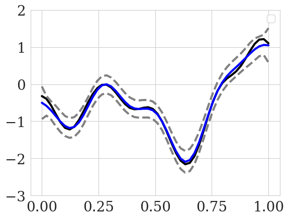
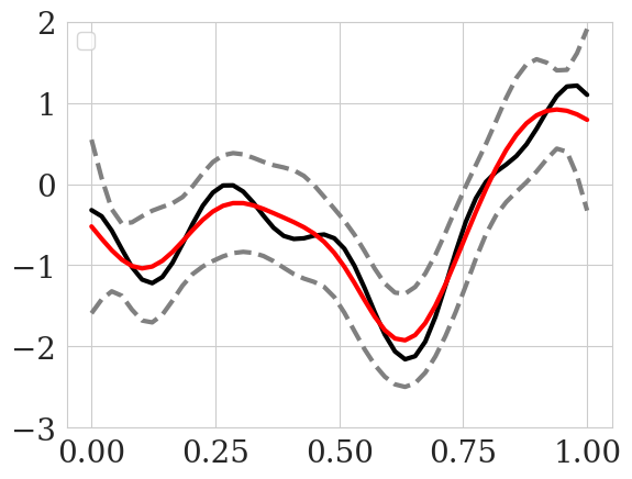
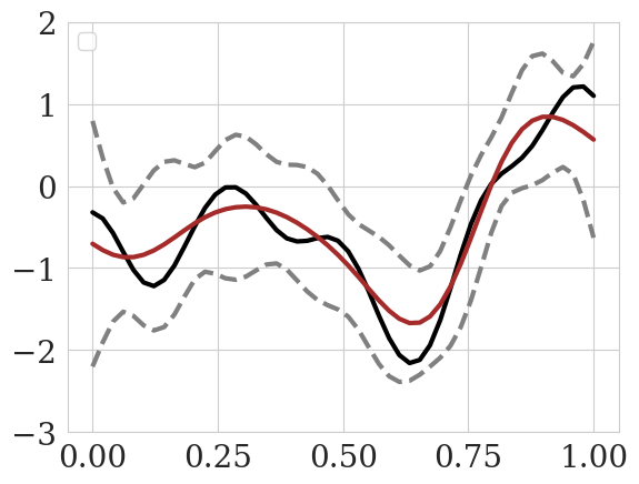
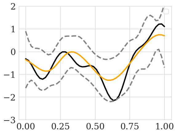
Figure 1: Posterior MCMC samples for the deblurring problem. From left to right: true posterior, free-form approximation, residual approximation and calibrated residual approximation. All methods use only $f$4 training points.

Comparison with GP regression-based approaches highlights that neural likelihood surrogates are significantly more data-efficient, achieving better accuracy than GP-based models even when the latter has access to ten times more training points.

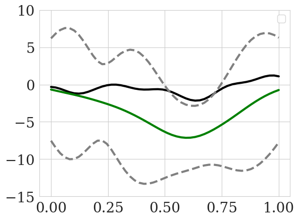
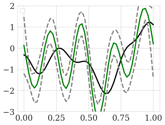
Figure 2: Posterior MCMC samples for the deblurring problem. From left to right: true posterior, GP regression with $f$5 training points and GP regression with $f$6 training points for the likelihood.

2. Nonlinear PDE-Based Imaging (Semiconductor Problem)

The framework is extended to a nonlinear PDE-based inverse problem: recovering the doping profile in a semiconductor from voltage-current measurements. Here, the forward mapping requires solving nonlinear Poisson and continuity equations, and the unknown is a spatially distributed parameter (modeled as a Gaussian random field).

Approximate NLLs (free-form, residual, calibrated residual) are trained from joint data, and posterior samples are compared against those from the true PDE-based model:

• Bias and variance of the posterior means for the free-form and residual NLLs are nearly identical to the exact PDE-based posterior, with $f$7 errors $f$8 and $f$9 versus $Z_f(y)$0 for the reference.
• Calibrated residual approximation degrades when the noise level is unknown, but the free-form remains robust.

Substantial computational gains are observed: likelihood evaluation via NLL surrogates is over $Z_f(y)$1 faster than PDE solves on the same hardware, and up to $Z_f(y)$2 faster when using parallel GPU evaluations.

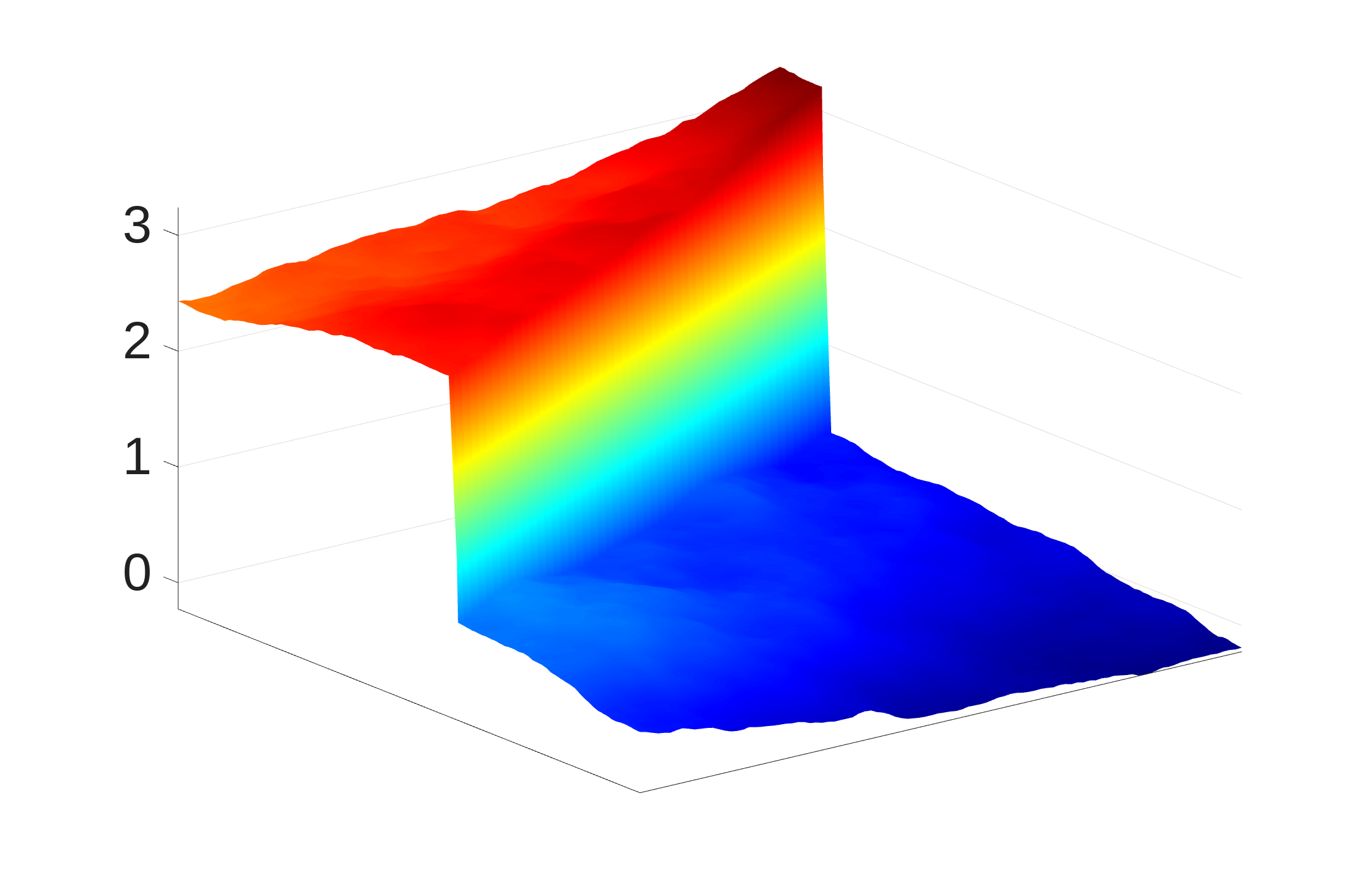
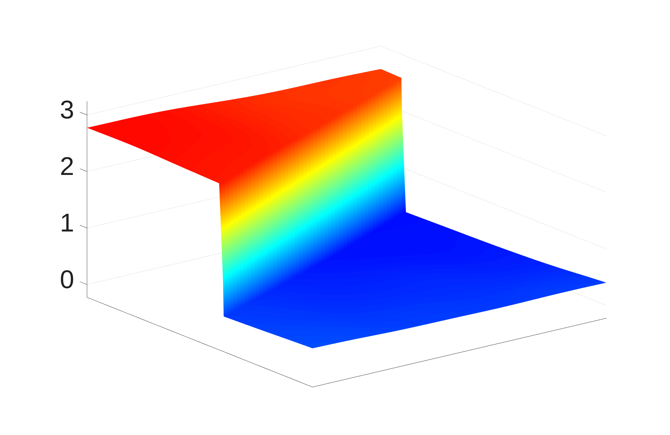
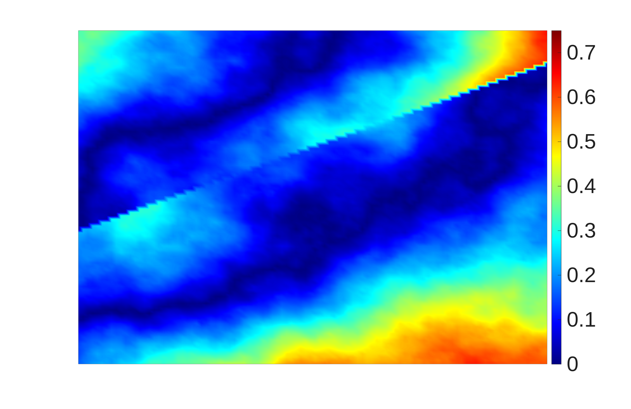
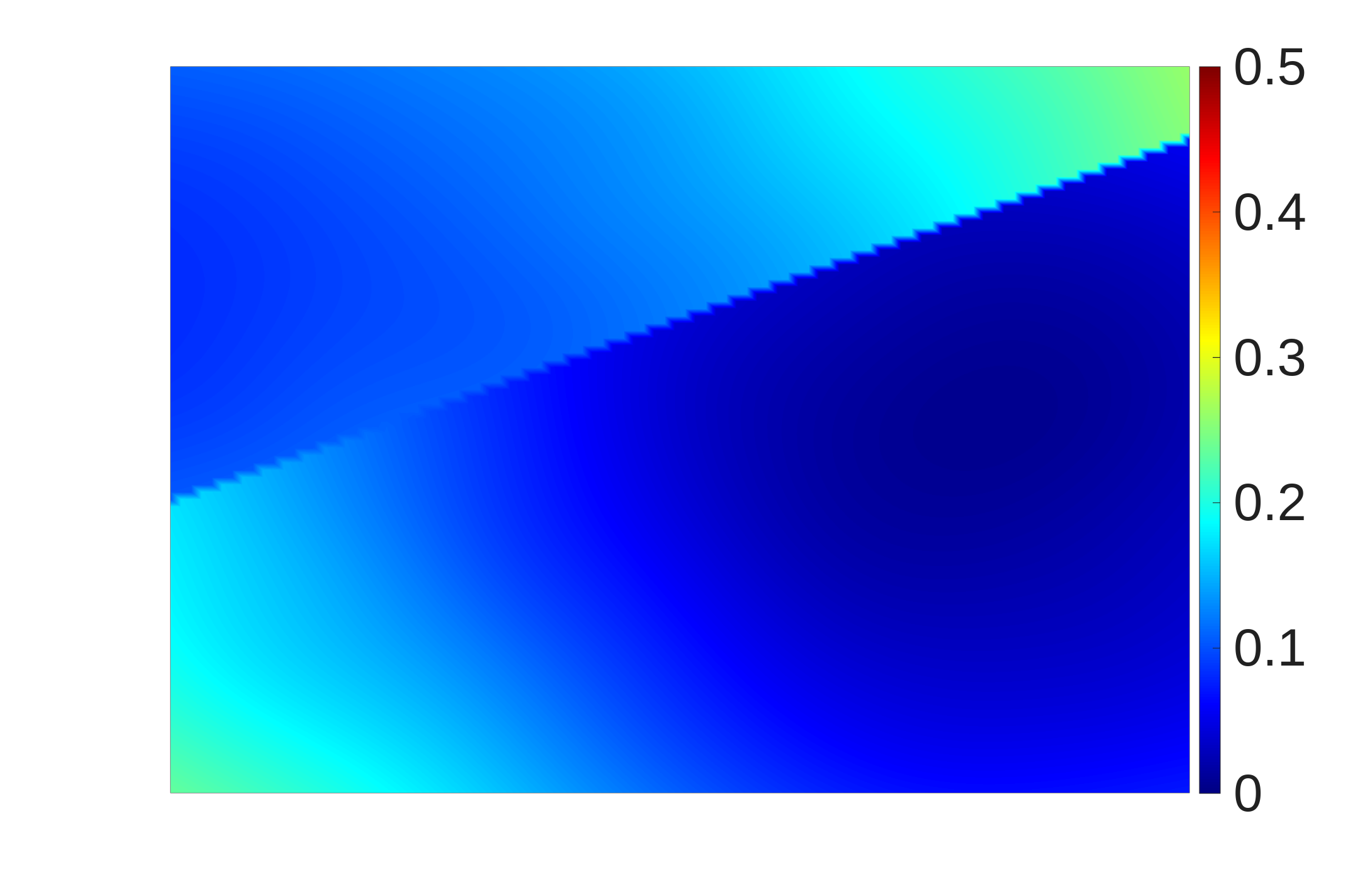
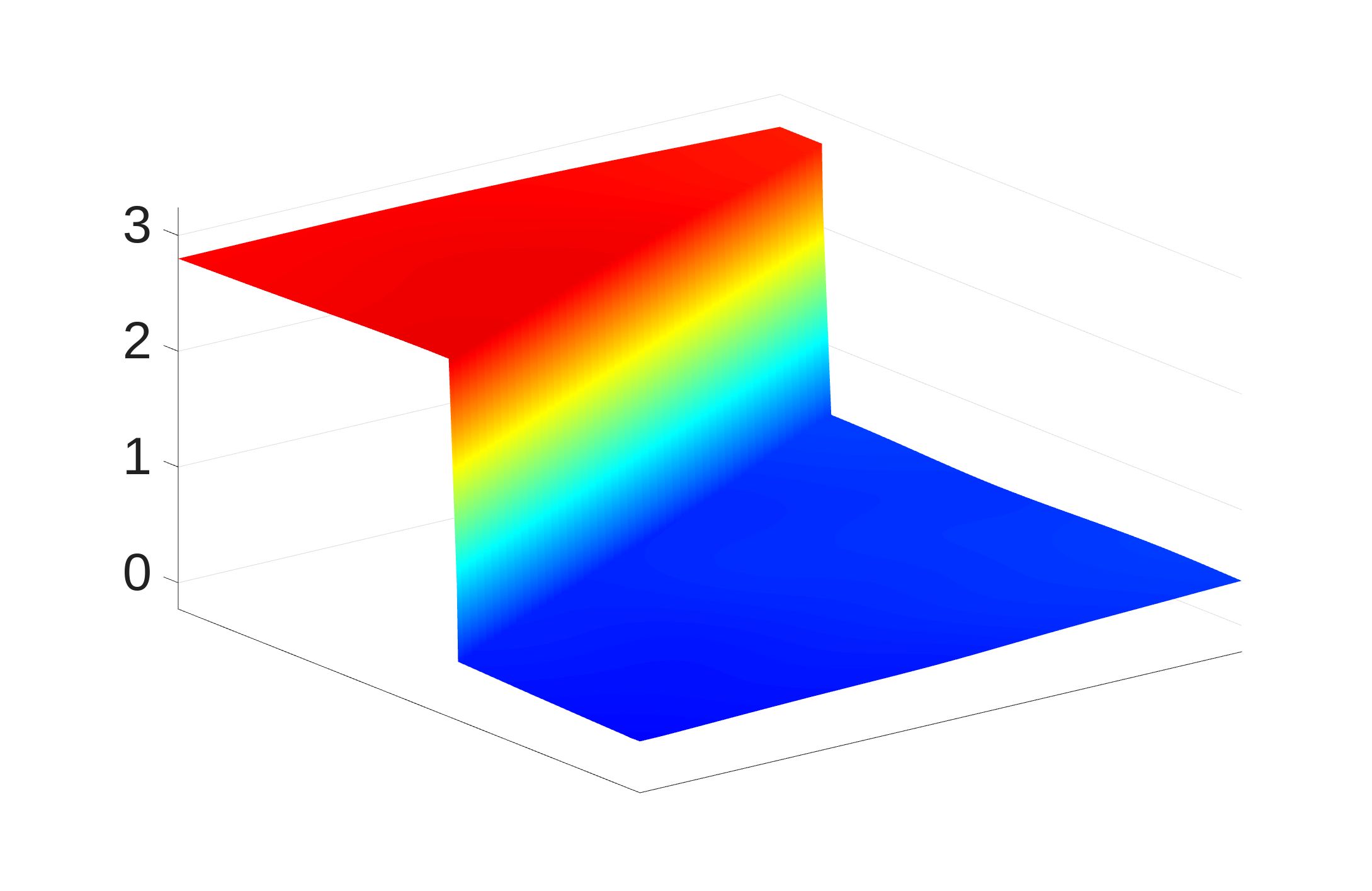
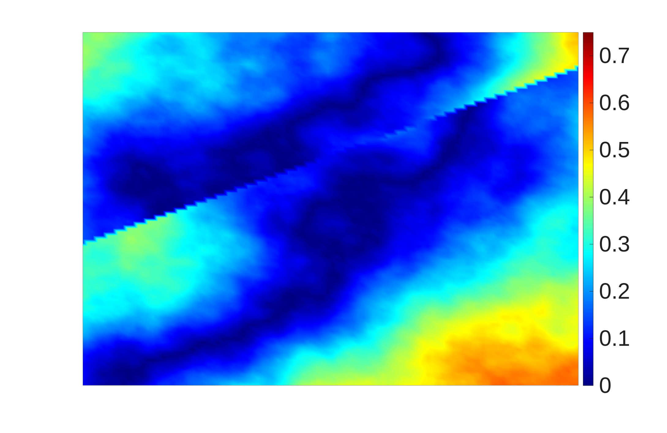
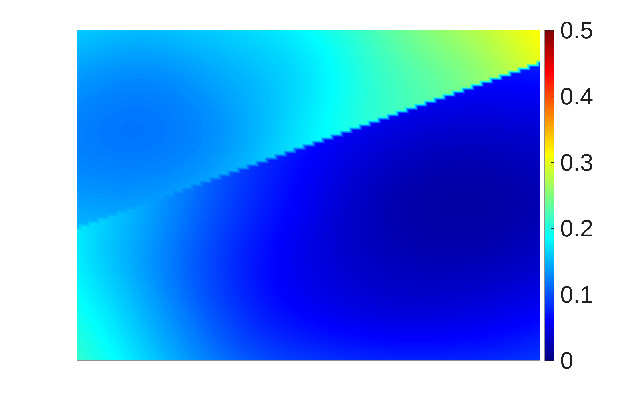
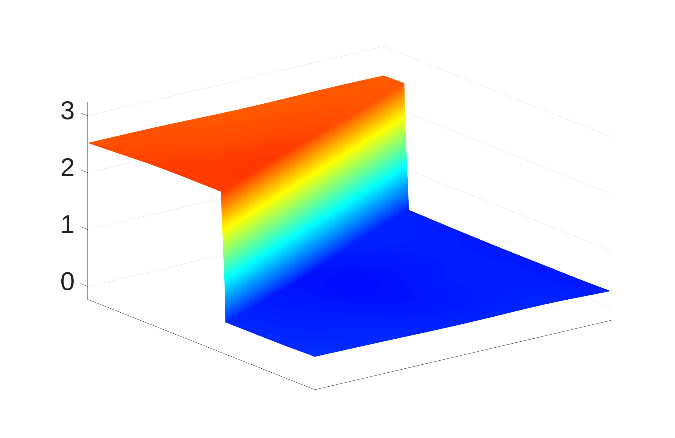
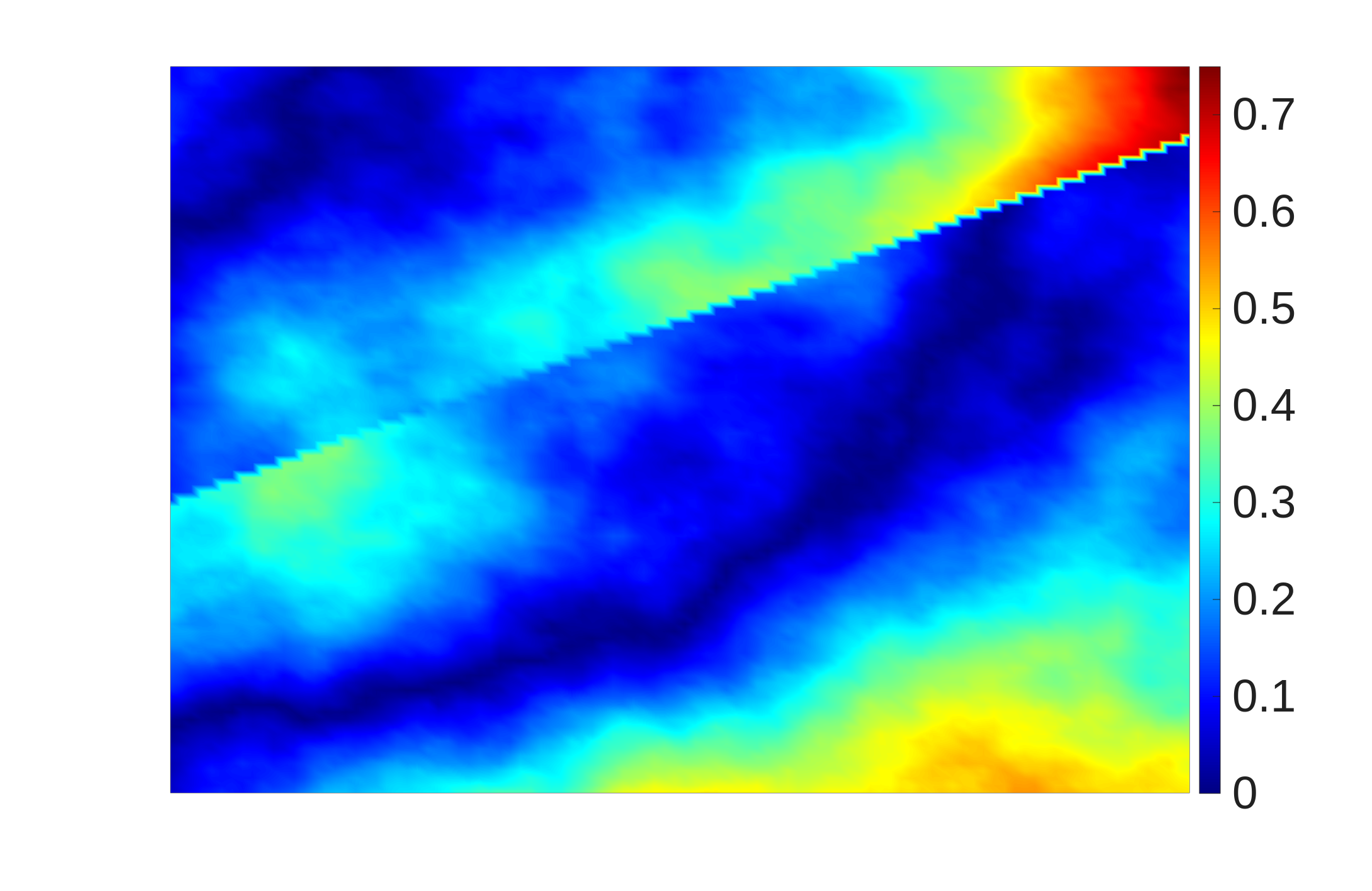
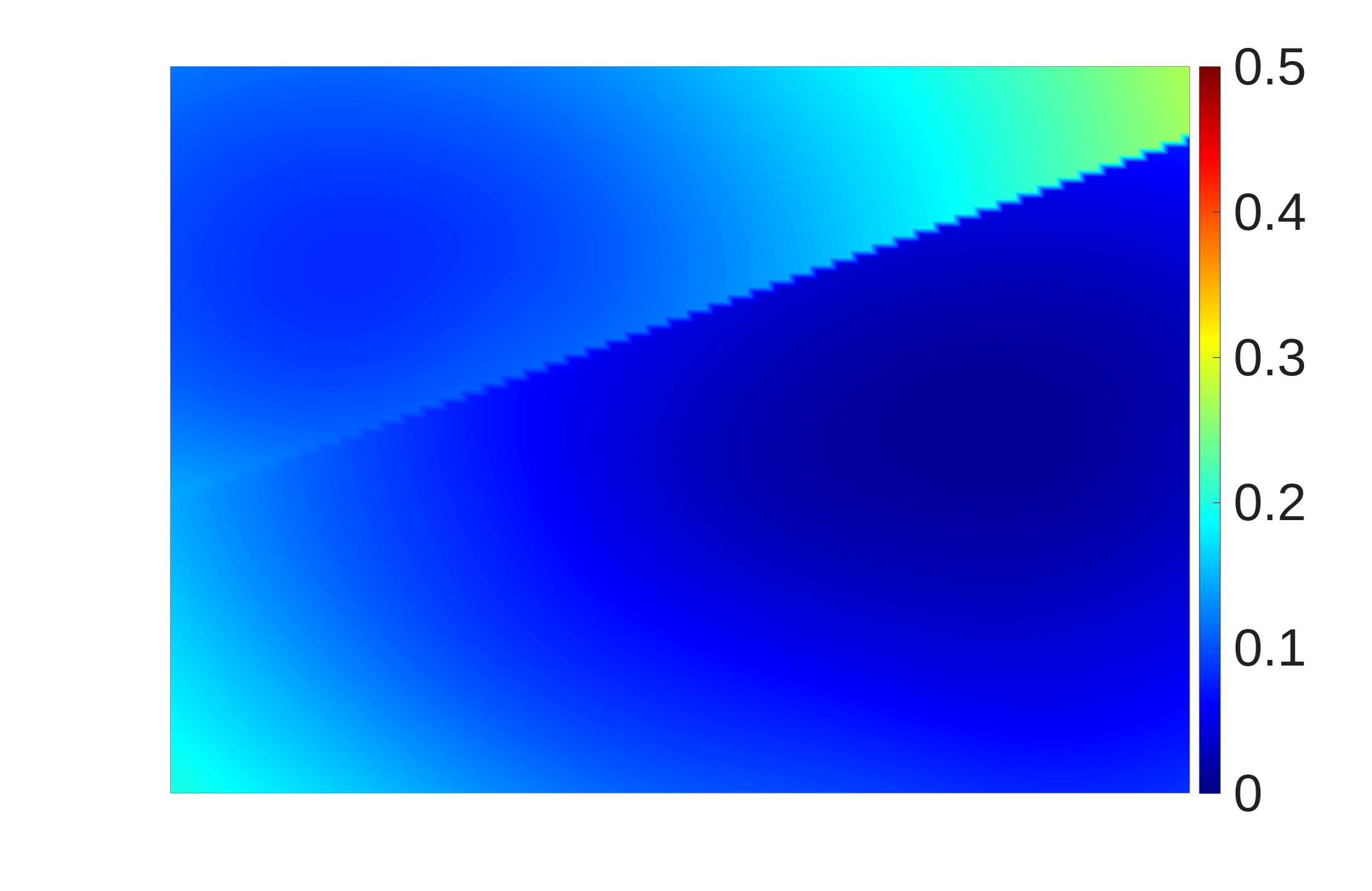
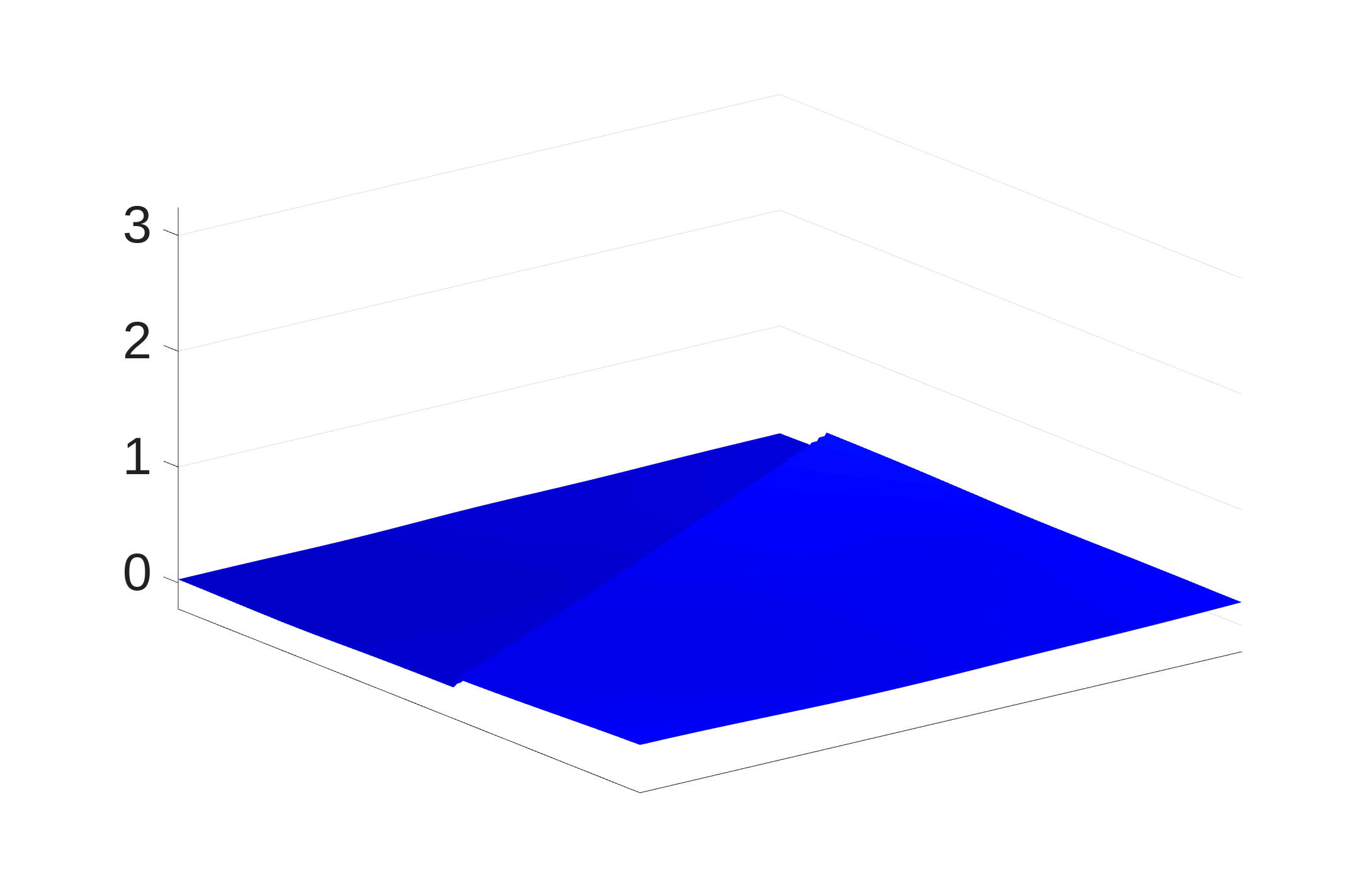
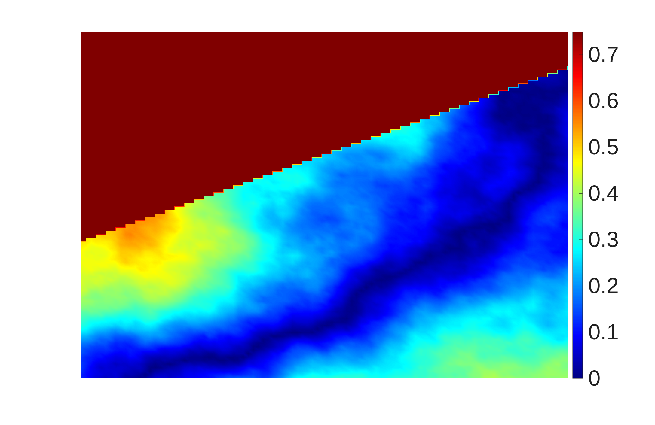
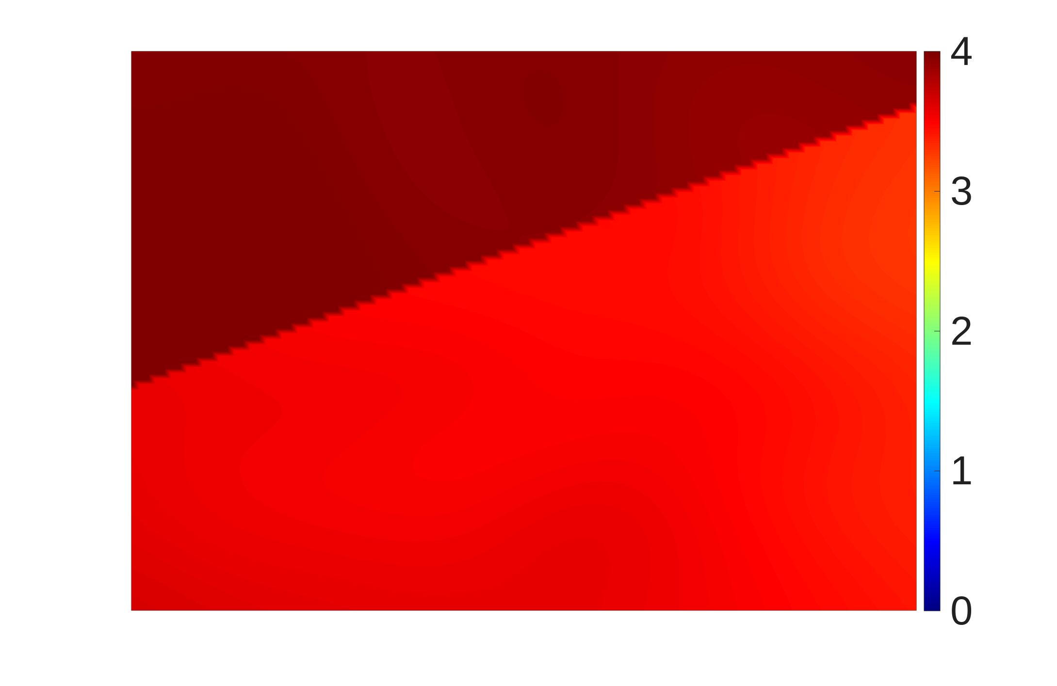
Figure 3: Summary of MCMC samples. Top row: True quantity of interest followed by posterior mean (left), bias (middle) and posterior variance (right) of the posterior samples with the true PDE-based NLL and its approximations. The $Z_f(y)$3 norm of the biases are $Z_f(y)$4 (exact), $Z_f(y)$5 (free-form), $Z_f(y)$6 (residual), $Z_f(y)$7 (calibrated residual).

Implications and Future Directions

This approach provides an efficient and theoretically well-founded workflow for data-driven Bayesian inference in high- or infinite-dimensional settings where explicit forward models or likelihoods may not be available. The avoidance of normalization bottlenecks permits the use of highly expressive function classes, and convexity ensures uniqueness and stability of solutions.

Potential future developments include:

• Extension of statistical consistency results to fully infinite-dimensional parameter spaces, leveraging further advances in empirical process theory.
• Quantitative convergence rates for surrogate learning, crucial for uncertainty calibration and sample complexity assessment.
• Integration with adaptive or online experimental design scenarios, where data generation and likelihood approximation could be intertwined.
• Application to additional domains such as geophysical imaging, inverse scattering, or high-dimensional biology, where empirical data is abundant but the physics is complex.

Conclusion

This work provides a significant advance in neural likelihood approximation for Bayesian inverse problems. By embedding normalization inside a KL-based convex objective defined over un-normalized potentials, the method unlocks the capacity to directly learn highly expressive, data-driven likelihood approximations—backed by strong guarantees of consistency and convexity. Empirical findings on both linear and nonlinear infinite-dimensional inverse problems validate its utility and efficiency, particularly in settings where classical likelihood- or flow-based surrogates are inapplicable.

Reference:

"A Convex Approximation Framework for Neural Likelihood-Based Bayesian Inverse Problems" (2607.06252)