TESSERA v2: Scaling Pixel-wise Earth Foundation Models
Abstract: Pixel-wise Earth-observation (EO) foundation models are now achieving state-of-the-art performance via generated spatial embeddings. However, how these models scale and how best to spend a pretraining budget remain poorly understood. We present the largest controlled scaling study for EO to date: 395 training runs on 1,024 GH200 superchips within a fixed pixel-wise Barlow Twins family, each evaluated on 15 downstream tasks. We find that pretraining loss barely predicts downstream performance (|Pearson r| < 0.2), so selecting models by loss wastes a large share of the compute. We also find that, as the training budget grows, the encoder and the data should grow together while the projector stays fixed, which gives a simple rule for allocating compute. Using this rule, we train a family of pixel-wise models (0.5B and 1B, with a 2B model in training) and distill them into compact students for embeddings-as-data deployment. The 21-million-parameter distilled TESSERA v2-1B-M in aggregate outperforms all open and proprietary models tested, some of which are orders of magnitude larger. These students produce Matryoshka representations that are inexpensive to serve: a 16-dimensional prefix keeps 92% of the full 128-dimensional performance at 1/8 of the storage. Upon completion of training we plan to release v2 global embeddings covering 2017-2025. Together, these results give a concrete, empirically grounded recipe for scaling pixel-wise EO foundation models: train large encoders, select by downstream performance, and distil into flexible student models. All code will be released at https://github.com/ucam-eo/tessera.
Paper Prompts
Sign up for free to create and run prompts on this paper using GPT-5.
Top Community Prompts
Explain it Like I'm 14
Overview: What this paper is about
This paper is about making satellite data easier and cheaper for everyone to use. The authors build and study “Earth embeddings,” which are short lists of numbers that summarize what’s happening at a small spot on Earth (a pixel) over time. These embeddings are made from satellites like Sentinel‑1 (radar) and Sentinel‑2 (optical), and can be used for lots of tasks—like mapping crops, spotting changes, or estimating population—without needing to process tons of raw images.
Their main goal is to figure out the best way to spend computing power when training these models, and then turn a big, powerful model into smaller, affordable versions that people can actually use at global scale.
Key questions the researchers asked
- If you have a fixed compute “budget,” what should you make bigger: the part of the model that reads data (the encoder), the part used only during training to shape the representation (the projector), or the amount of training data?
- Is the training score (called “loss”) a good way to choose the best model, or should we choose based on how well the model actually works on real tasks?
- Can we train one large model and then compress its knowledge into small models that keep most of the quality but are much cheaper to run and store?
- Can we offer embeddings in different sizes (like 16, 32, 64, or 128 numbers per pixel) so users can pick the right trade‑off between accuracy and storage?
How they approached the problem (in everyday language)
Think of this like building a team to study Earth from space:
- The encoder is the “expert reader”: it looks at satellite time series for each pixel and learns a smart summary (the embedding).
- The projector is a training helper: it shapes the embeddings while learning but isn’t needed later when the model is used.
- The embedding is the “ID card” for a place and time: a short list of numbers that captures important details (like patterns of vegetation over the year).
What they did:
- Ran a giant, controlled test: 395 different training runs on powerful GPUs, changing only three things—encoder size, projector size, and how much training data they used—so they could see how each one affects results. Each model was evaluated on 15 real tasks (like classification, segmentation, regression).
- Compared two ways to pick models:
- By training loss (like how well they did on practice drills).
- By downstream performance (how well they perform on real jobs).
- Found a “recipe” for using compute wisely:
- Grow the encoder and the dataset together as you have more compute.
- Keep the projector small and fixed.
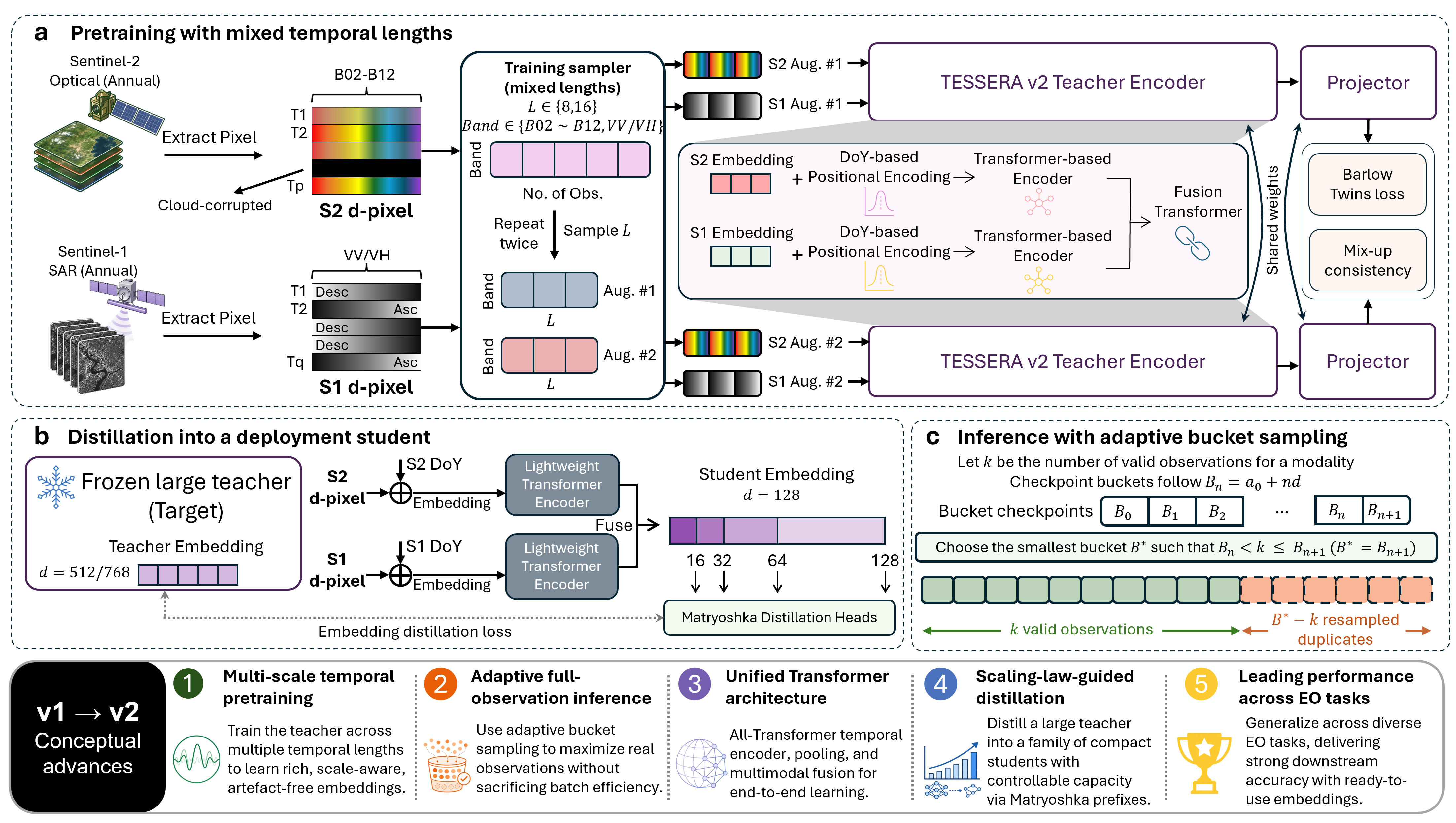
- Trained a big “teacher” model (about 1 billion parameters), then used knowledge distillation (a teacher-student method) to train smaller “student” models that are easier to use and deploy.
- Made “nested embeddings”: from the same 128‑number embedding, you can use just the first 16, 32, or 64 numbers if you need to save storage—and it still works well.
Helpful analogies:
- Training loss vs. downstream performance is like practice scores vs. game scores: being great at drills doesn’t always mean you’ll win real games.
- Distillation is like a top student explaining a topic to juniors: the juniors learn to give very similar answers, faster and more efficiently.
- Nested embeddings are like a summary at different lengths (1‑page, 2‑page, 4‑page, full report): shorter versions keep most of the key points.
Key terms (in simple words):
- Embedding: a compact set of numbers that describe a place and time.
- Encoder: the model part that reads satellite data and produces embeddings.
- Projector: a training‑time helper that shapes the embeddings; not used in deployment.
- Distillation: training a small model to mimic a large model’s outputs.
- Downstream tasks: real problems we care about (e.g., crop mapping).
- “Embeddings‑as‑data”: precomputing embeddings and sharing them as ready‑to‑use map layers so users don’t need big GPUs.
Main findings and why they matter
- Training loss barely predicts real‑world performance
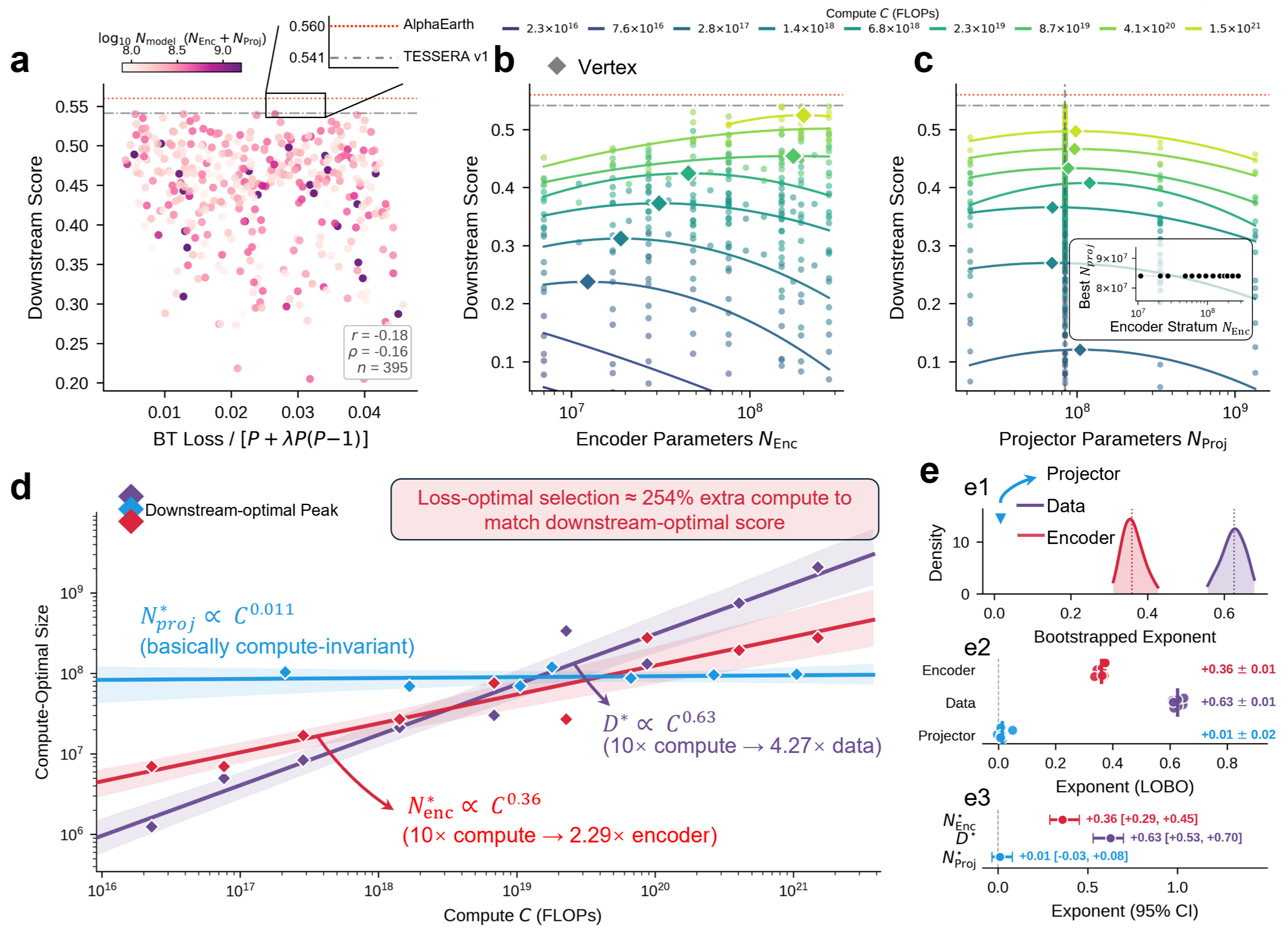
- Across 395 runs, training loss and downstream task scores were only weakly related.
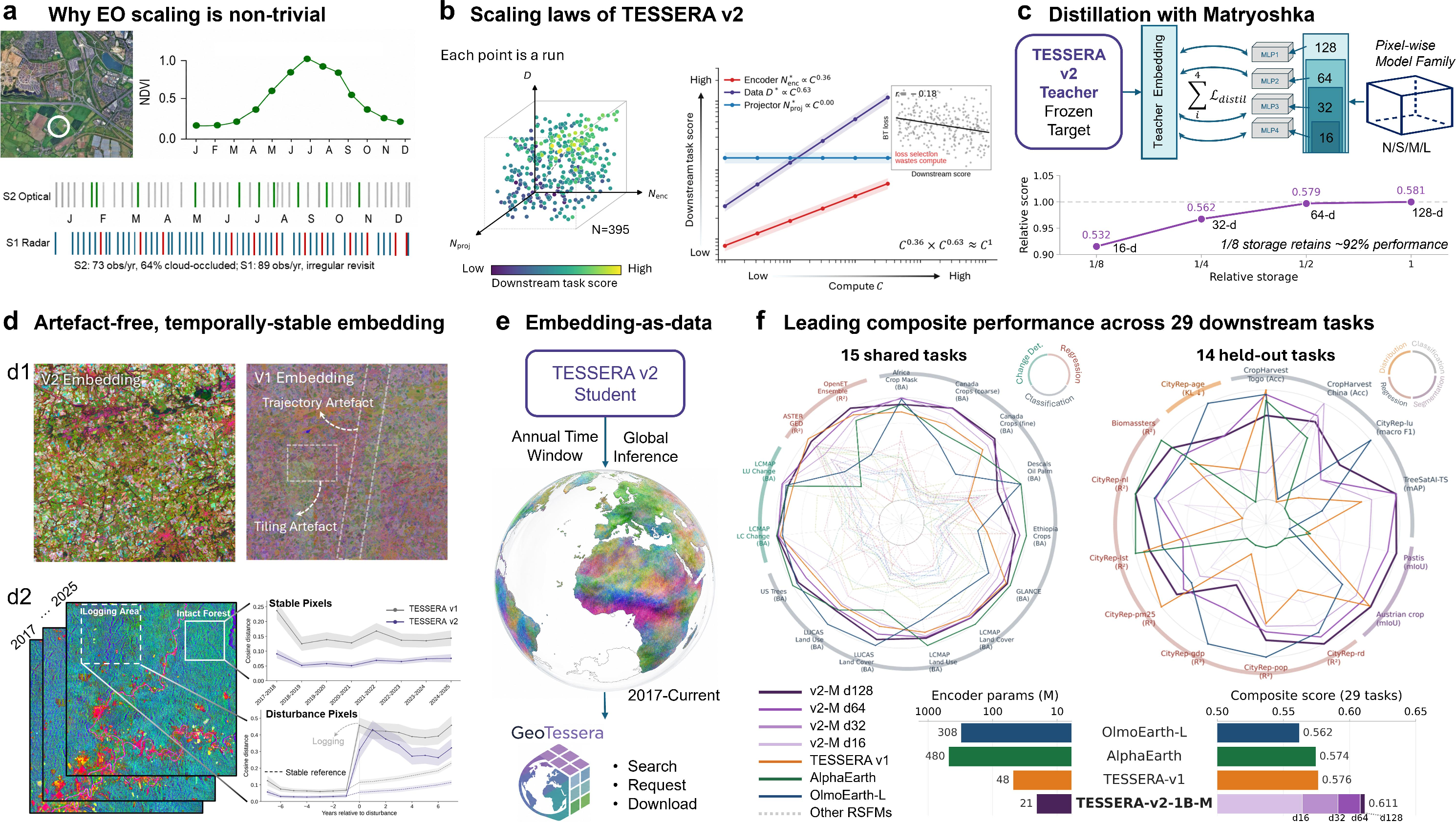
- Picking models by training loss led to wasting a lot of compute (around 3× more) compared to picking by real task performance.
- Why it matters: In Earth data, things like clouds and irregular satellite visits can trick the training score. So you should pick models based on how they perform on actual tasks, not just on a low training loss.
- Spend your compute on the encoder and data, not the projector
- As compute increases, the best results come from growing:
- the encoder (the part that “understands” the data), and
- the amount of training data,
- while keeping the projector size about the same.
- Why it matters: This gives a simple rule for future training—build bigger, better “readers” and feed them more data; don’t waste compute on a larger projector.
- As compute increases, the best results come from growing:
- Big teacher, small students: best of both worlds
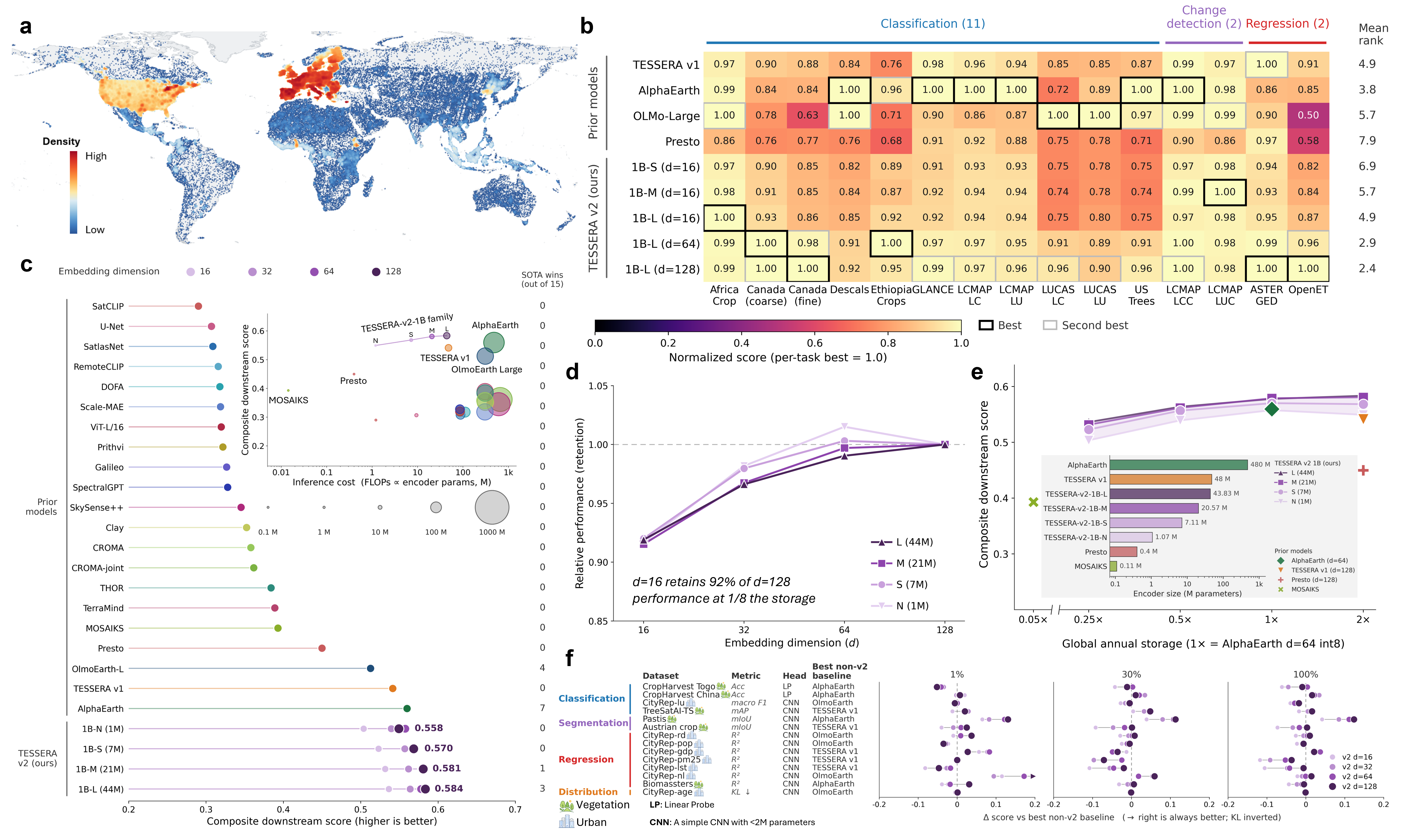
- They trained a large 1B‑parameter teacher model and distilled it into smaller student models (from ~1M to ~44M parameters).
- The mid‑sized 21M student (v2‑1B‑M) outperformed other open and proprietary systems on a 29‑task suite (15 core tasks + 14 new ones), despite being much smaller and cheaper to use.
- Storage‑friendly nested embeddings work really well
- The 16‑number version kept about 92% of the accuracy of the full 128‑number version but used only 1/8 of the storage.
- This makes it easy to choose a version that fits your storage and internet limits without retraining.
- Cleaner, more stable embeddings over time
- The new embeddings reduce “artefacts” like striping and seams from satellite acquisition.
- They are more stable from year to year when nothing changes on the ground, and they recover better after temporary disturbances.
What this means for the future
- Clear training guidance: If you’re building Earth‑observation models, don’t rely on training loss to choose the winner. Test on real tasks. Spend your compute on larger encoders and more data; keep the projector small.
- Practical products: People can use these embeddings as ready‑to‑download data, with flexible sizes (16, 32, 64, 128 numbers) to save storage and bandwidth.
- Lower barriers: Users don’t need big GPUs or deep remote‑sensing expertise. They can train small “heads” on top of embeddings for their specific tasks.
- Bigger impact: Better, cheaper, and more flexible Earth data can help in agriculture, climate monitoring, city planning, ecology, and more.
- Open science: The team plans to release global embeddings for 2017–2025 and the code, helping others build on this work.
In short, the paper offers a simple, evidence‑based strategy: train a big encoder with lots of data, pick models by how well they do on real tasks, and distill that knowledge into small, flexible embeddings that are easy for everyone to use.
Knowledge Gaps
Knowledge gaps, limitations, and open questions
Below is a single, concrete list of unresolved issues and open directions that future researchers could act on:
- External validity of the scaling laws: verified only for pixel-wise Sentinel‑1/2 encoders with a redundancy-reduction objective; needs replication for other objectives (contrastive, masked modeling), patch-based and multi-resolution architectures, and broader multimodal settings.
- Loss-to-downstream reliability: no theory or alternative proxy is proposed to replace the weakly predictive pretraining loss; need selection metrics that correlate with downstream performance without full task evaluation.
- Projector invariance: conclusion that projector size need not scale is based on one projector design and four widths; requires testing deeper/wider projectors, different normalizations, and objectives to confirm generality.
- Compute–data–epochs disentanglement: teacher trained for one epoch and sweep fits assume a fixed training regime; need experiments varying training tokens/epochs to separate under/over-training effects across sizes.
- Hyperparameter sensitivity: scaling conclusions were derived under fixed optimizers, LR schedules, augmentations, and batch sizes; robustness to these choices is untested.
- Data scaling regime: the sweep spans 0.03–9,984M samples and the teacher uses ~4.2B dpixels; need to map where diminishing returns start and how token budgeting interacts with model capacity.
- Temporal granularity of the product: embeddings are annual; open whether quarterly/monthly or multi-scale temporal embeddings improve tasks requiring intra-annual dynamics (e.g., phenology, crop stages, fast-onset events).
- Inference bucketization effects: midpoint resampling and bucket sizes are heuristic; no quantitative analysis of biases introduced across climates, sparse series, or extreme sampling irregularity.
- Robustness to missing modalities: performance where Sentinel‑2 is persistently cloudy or where Sentinel‑1 is absent is not quantified; need systematic evaluation and fallback strategies with associated quality flags.
- Geographical and climatic coverage: benchmarks skew to well-studied regions; require evaluation across under-represented biomes (e.g., polar night, deserts, high latitudes, tropical cloud belts) and culturally/geopolitically diverse areas.
- Temporal robustness and drift: inter-annual stability is shown qualitatively; need quantitative stability metrics across 2017–2025, sensitivity to sensor reprocessing, and long-term drift analyses.
- Sensor generalization and fusion: approach is limited to Sentinel‑1/2; integrating Landsat 8/9, Sentinel‑3, MODIS/VIIRS, PlanetScope, commercial SAR, and thermal data—and re-testing the scaling rules—remains open.
- Spatial resolution transfer: embeddings are produced at 10 m; unclear how methods and scaling behavior extend to 3–5 m or 30 m data and whether embeddings transfer across resolutions.
- Interpretability and physical alignment: no probing to link embedding dimensions to geophysical variables (e.g., NDVI, biomass, soil moisture) or to detect spurious correlations; actionable interpretability studies are missing.
- Uncertainty and quality metadata: embeddings are deterministic without per-pixel uncertainty or reliability scores; methods to estimate and serve uncertainty/quality flags are needed.
- Distillation design space: only cosine reconstruction with linear prefix heads is explored; need ablations with MSE/KL losses, temperature scaling, intermediate feature matching, and teacher projector supervision.
- Prefix monotonicity and task-specific degradation: global “graceful degradation” is reported, but per-task monotonicity guarantees and identification of tasks that degrade sharply at low dimensions are not provided.
- Teacher–student dimensionality choices: the impact of teacher embedding size (T=768) on student performance/efficiency is unstudied; optimal teacher dimensionality and compression ratios are unknown.
- Negative transfer across tasks: a single embedding supports diverse tasks; need analyses of task conflicts and strategies (e.g., multi-head adapters, task-conditioned readouts) to mitigate negative transfer.
- Head capacity dependence: downstream evaluation uses small fixed heads; it remains unclear how rankings change with stronger heads, linear probing, or light fine-tuning.
- Storage/IO and precision: dimension prefixes address storage but numeric precision (e.g., fp16 vs int8) and compression are not systematically evaluated; need quantization and I/O throughput studies.
- Update cadence and versioning: release plan for 2017–2025 embeddings lacks details on update strategy, backward compatibility, and handling upstream reprocessing changes (e.g., L2A algorithm updates).
- Energy and carbon footprint: the cost of 395 runs and teacher training is high; energy/CO2 accounting and methods to reduce environmental impact per unit downstream utility are not provided.
- Reproducibility gaps in the sweep: full details of the architectural pre-sweep (7 axes), random seeds, and exact configs are not presented; independent replication across hardware clusters remains unverified.
- Out-of-distribution (OOD) stress tests: performance on rare/extreme events (wildfires, floods, volcanoes, hurricanes) and abrupt land-cover changes is not reported; OOD robustness and false-positive rates in change detection need assessment.
- Distillation sampling strategy: ~200M dpixels used for distillation, but sampling scheme is unspecified; stratified, bias-aware sampling and its effect on student generalization should be studied.
- Product-level metadata: how tiling, indexing, cloud masks, and data provenance are served with embeddings is unspecified; standards for metadata to support reliable downstream use are needed.
- Ethical/governance considerations: beyond a brief ethics statement, there is no assessment of misuse risks (e.g., surveillance), sensitive-location handling, or governance frameworks for open embeddings.
- Security/privacy: potential for de-anonymization or inference of sensitive attributes from embeddings is not discussed; threat models and mitigations are missing.
- Theoretical account of exponents: observed exponents (encoder ~C0.36, data ~C0.63, projector ~C0) lack a mechanistic explanation; theory to explain when and why projector capacity should remain fixed is an open problem.
- Cheaper model-selection proxies: since downstream evaluation is costly, discovering low-cost proxies (e.g., curated probes, synthetic tasks, linear transfer metrics) for model selection is an open need.
- Continual/online updates: methods to incrementally update embeddings with new data/sensors without reprocessing all years (e.g., streaming distillation, rehearsal buffers) are unexplored.
Practical Applications
Overview
This paper presents downstream-driven scaling laws and a deployable “embeddings-as-data” family (TESSERA v2) for pixel-wise Earth Observation (EO) using Sentinel-1/2. Key findings and innovations with practical impact include:
- A compute-allocation rule: spend pretraining budget on encoder capacity and data, keep the projector size fixed; select models by downstream performance rather than pretraining loss.
- A high-capacity teacher distilled into compact students (N/S/M/L) with storage-adaptive embedding prefixes (16/32/64/128 dims) that preserve most performance at lower storage/IO cost.
- Analysis-ready global annual embeddings (10 m) intended for 2017–2025, reducing the need for raw imagery processing and user-side GPU inference.
Below are actionable applications organized by time horizon. Each bullet highlights sectors, potential tools/products/workflows, and assumptions/dependencies affecting feasibility.
Immediate Applications
- Land cover mapping and updates (classification/segmentation)
- Sectors: government, environmental NGOs, geospatial SaaS, consulting
- Tools/workflows: use TESSERA v2 embeddings as features; train a small MLP/CNN head per region; deploy different prefixes (e.g., d=16 for quick scans, d=64/128 for production); integrate via STAC/Cloud-Optimized GeoTIFF + PostGIS/QGIS
- Assumptions/dependencies: annual cadence; 10 m spatial resolution; coverage 2017–2025; better performance in well-represented regions/tasks similar to AlphaEarth
- Agricultural monitoring (crop type, phenology proxies, field boundary delineation, yield-related regression)
- Sectors: agriculture/AgTech, food security, insurance
- Tools/workflows: low-label training of small heads on v2 embeddings; use d=64 for regression-heavy tasks; integrate with farm management systems; support in-season analytics from prior-year patterns
- Assumptions/dependencies: annual embeddings (not intra-seasonal); Sentinel-1/2-derived features may miss crop-specific phenology at sub-annual scale; regional label availability affects head performance
- Forestry and nature-based solutions MRV (deforestation, degradation, tree species proxies, biomass)
- Sectors: forestry, carbon markets, conservation finance, ESG
- Tools/workflows: change-detection heads comparing annual embeddings; dashboards for project monitoring; compact prefixes (d=16) for wide-area scans, d=64/128 for verification
- Assumptions/dependencies: annual temporal granularity; calibration to local forest types may be needed; biomass estimation needs careful head design and ground truth
- ESG and supply-chain due diligence (e.g., EU Deforestation Regulation compliance)
- Sectors: finance, retail/CPG, commodity traders
- Tools/workflows: site-level monitoring using embeddings; similarity search over embeddings for risk screening; alerts on land-cover change in supplier polygons
- Assumptions/dependencies: accurate supplier geofencing; annual granularity may delay detection; jurisdiction-specific thresholds and legal standards
- Insurance risk and claims analytics (hazard/asset exposure, parametric triggers for land-surface change)
- Sectors: insurance/reinsurance, catastrophe modeling
- Tools/workflows: precompute embeddings over portfolios; build per-peril heads (e.g., burn scars, flood-related land-surface change); store d=32/64 to balance accuracy vs. storage
- Assumptions/dependencies: indirect hazard proxies from land surface; annual cadence limits immediate post-event use; complementary event-detection data likely required
- Urban growth and infrastructure mapping (land-use, road density, informal settlement dynamics)
- Sectors: urban planning, municipal governments, infrastructure funds, mobility
- Tools/workflows: lightweight heads for land-use and density metrics; integrate into planning GIS; rapid “what’s changed since last year” layers using two-year embeddings
- Assumptions/dependencies: annual embeddings limit detection of short-term construction events; accuracy may vary with urban morphology
- Conservation planning and biodiversity habitat proxies
- Sectors: conservation NGOs, biodiversity credits, protected area management
- Tools/workflows: habitat classification heads; corridor and fragmentation metrics built from embeddings; compact prefixes enable regional-scale analyses on limited storage budgets
- Assumptions/dependencies: proxies for habitat often need ancillary data (DEM, climate, species records); annual cadence OK for many habitat use-cases
- Water resources and agriculture water-use proxies (surface water extent, irrigated area, drought indicators)
- Sectors: water agencies, agriculture, NGOs
- Tools/workflows: binary/continuous heads for water extent and irrigation proxies; combine SAR+optical embeddings for cloudy regions; deploy d=64 for better regression fidelity
- Assumptions/dependencies: annual cadence misses short-lived water events; local validation advisable
- Disaster impact baselines and recovery tracking (e.g., burn scars, long-term urban/rural recovery)
- Sectors: emergency management, donors, development banks
- Tools/workflows: annual before/after embeddings for medium- and long-term recovery indicators; integrate with external rapid-response datasets for near-real-time needs
- Assumptions/dependencies: not a substitute for rapid mapping; optimal for medium-term assessments
- Geospatial ML productivity and MLOps
- Sectors: software/ML platforms, RSFM builders, academia
- Tools/workflows: adopt the paper’s compute allocation recipe (scale encoder+data, keep projector fixed); use downstream task metrics for model selection; distill teachers to size-tiered students; build internal embedding feature stores with prefix choices to control storage/IO
- Assumptions/dependencies: access to large-scale compute for pretraining is not required for users consuming embeddings; for builders, significant compute/data engineering remains necessary
- Geospatial similarity search and “geo-RAG”
- Sectors: consulting, environmental analytics, site selection
- Tools/workflows: index embeddings in a vector database for “find places like X” workflows; plug into analytical notebooks and dashboards for analog-based reasoning
- Assumptions/dependencies: annual embeddings encode multi-sensor context but not sub-annual events; appropriate distance metrics and domain calibration advised
- Education and workforce upskilling in EO/RS
- Sectors: education, capacity building, public sector
- Tools/workflows: use embeddings in teaching labs to avoid heavy preprocessing; small heads illustrate classification/regression/change-detection; vary prefix to demonstrate accuracy/storage trade-offs
- Assumptions/dependencies: internet/storage access to embedding tiles; basic Python/GIS skills
- Edge/low-resource deployments on small AOIs
- Sectors: field operations, NGOs, local governments
- Tools/workflows: run the N/S student locally for small regions if raw S1/S2 are available; or consume precomputed embeddings where bandwidth is constrained by using d=16/32
- Assumptions/dependencies: on-device inference still requires access to and preprocessing of raw S1/S2 unless precomputed embeddings are used; performance/coverage depends on data availability
Long-Term Applications
- Higher-frequency monitoring and alerts (sub-annual or near-real-time change detection)
- Sectors: forestry, disaster response, compliance monitoring
- Tools/workflows: extend embeddings to monthly/quarterly windows; push incremental updates; automated alerts for deforestation, flooding, or construction
- Assumptions/dependencies: requires retraining/inference at higher cadence and more storage/compute; handling clouds and irregular revisits becomes more critical
- Multi-sensor, multi-resolution fusion beyond Sentinel-1/2
- Sectors: national mapping, commercial EO, defense/civil protection
- Tools/workflows: integrate Landsat, Sentinel-3, L-band SAR, commercial optical/SAR; retrain teacher with expanded data; distill into students with consistent prefixes
- Assumptions/dependencies: licensing for commercial data; harmonization challenges; additional compute
- National to global policy dashboards for climate adaptation and land governance
- Sectors: public policy, development agencies, regulators
- Tools/workflows: embed annual indicators (land-cover transitions, vegetation condition, urban expansion) into open dashboards; standardize MRV for programs and regulations
- Assumptions/dependencies: governance frameworks and standard definitions; ground validation; sustainable funding for updates
- Energy systems planning and operations (renewable siting, grid expansion, encroachment risk)
- Sectors: energy/utilities, transmission operators
- Tools/workflows: combine embeddings with wind/solar resource and grid data for site screening; monitor vegetation encroachment or land-use constraints along corridors
- Assumptions/dependencies: operational forecasting needs finer temporal resolution; integration with utility asset databases
- Environmental health and epidemiology (vector-borne disease risk, urban heat exposure)
- Sectors: public health, NGOs, academia
- Tools/workflows: use embeddings as environmental covariates in risk models; annual baselines for long-term exposure/inequity studies; detect persistent heat islands and greenspace deficits
- Assumptions/dependencies: needs health outcomes and socio-demographic data; temporal alignment and causal interpretation care
- Finance and macro nowcasting (economic activity proxies, ESG/impact tracking)
- Sectors: asset management, sovereign risk, development finance
- Tools/workflows: train heads to nowcast GDP, nighttime lights, road/building density, or productivity proxies; portfolio-level E, S tracking over space and time
- Assumptions/dependencies: careful validation to avoid spurious correlations; regulatory constraints on model use; annual cadence limits short-term trading
- Digital twins and planning simulations
- Sectors: smart cities, infrastructure, climate resilience
- Tools/workflows: plug embeddings into digital twin platforms as consistent environmental layers; scenario analysis for land-use policies and climate adaptation
- Assumptions/dependencies: interoperability with 3D/temporal twin stacks; higher-frequency updates desirable
- Robotics and field autonomy context layers
- Sectors: agriculture robotics, environmental monitoring, logistics
- Tools/workflows: use embeddings as prior context for route planning, habitat avoidance, or crop/land-cover priors
- Assumptions/dependencies: real-time operation requires higher temporal resolution and local sensing; integration with onboard perception
- Data-centric Earth system modeling and assimilation
- Sectors: climate/land-surface modeling, hydrology
- Tools/workflows: embeddings as compact observational features in data assimilation or hybrid AI–physics models; bias-correction via learned heads
- Assumptions/dependencies: methodological development for assimilation of high-dimensional learned features; physical interpretability
- Low-code/AutoML geospatial analytics
- Sectors: software platforms, enterprise analytics
- Tools/workflows: wrap embeddings + lightweight heads in AutoML pipelines (Vertex AI/SageMaker plug-ins); template recipes for common tasks (LCM, change detection, parcel mapping)
- Assumptions/dependencies: platform integrations; responsible defaults for regions with limited representation
- Responsible AI and domain adaptation toolkits
- Sectors: academia, NGOs, regulators
- Tools/workflows: bias audits and adaptation methods for underrepresented climates/seasons; uncertainty quantification on embedding-driven predictions
- Assumptions/dependencies: requires curated benchmarks in under-sampled geographies; additional labels for calibration
Cross-Cutting Assumptions and Dependencies
- Data scope: current model family is trained on Sentinel-1/2; embeddings are annual at 10 m for 2017–2025. Tasks needing sub-annual insights or other modalities may require extensions.
- Generalization: strongest performance is shown on AlphaEarth and related tasks; underrepresented climates/seasons/regions may need domain adaptation or additional labels.
- Compute/storage: embeddings reduce user-side GPU needs but still require storage/IO proportional to dimension; the prefix mechanism (d=16/32/64/128) provides a practical knob.
- Tooling: practical use benefits from easy retrieval libraries, GIS plugins, and feature-store integrations; code and embeddings are planned for release at https://github.com/ucam-eo/tessera.
- Governance: policy and ESG use-cases require clear definitions, validation protocols, and alignment with regulatory standards.
Glossary
- AlphaEarth: A benchmark suite of Earth observation tasks and datasets used to evaluate embeddings and models. "Across a $29$-task suite (the $15$-task AlphaEarth plus $14$ further held-out datasets)"
- analysis-ready: Data prepared so it can be used directly without additional preprocessing or inference. "It should be analysis-ready, giving users a geospatial data layer they can work on directly, without processing raw imagery or running GPU inference."
- along-track striping: Striped artefacts aligned with satellite acquisition tracks visible in imagery or embeddings. "v1 embeddings often show along-track striping and tile-seam discontinuities aligned with Sentinel-2/Sentinel-1 acquisition geometry."
- attention pooling: Aggregating sequence features by learned attention weights. "aggregates the variable-length sequence by learned attention pooling."
- bf16: Bfloat16, a 16-bit floating-point format with an 8-bit exponent used to improve training efficiency and stability. "under FSDP in bf16."
- bootstrap: A resampling method for estimating stability or uncertainty in fitted parameters. "Bootstrap and leave-one-bucket-out stability of the three exponents."
- chance-adjusted metrics: Evaluation metrics normalized to account for chance-level performance. "with chance-adjusted metrics: for classification and for regression."
- change detection: Tasks that identify changes over time in imagery or embeddings. "classification, segmentation, regression, and change detection."
- cloud and shadow masking: Identifying and masking cloud and shadow pixels to avoid contamination in remote-sensing data. "radiometric calibration, cloud and shadow masking, cross-sensor harmonisation, and expensive computation over raw imagery."
- cloud-free composites: Temporal composites of imagery selecting cloud-free observations. "and the cloud-free composites most models train on remove the phenological dynamics that downstream tasks depend on"
- compute-optimal: The configuration that yields the best performance for a given compute budget. "vertices mark compute-optimal sizes per compute bucket."
- cross-modal fusion: Combining multiple data modalities (e.g., optical and SAR) within a model to produce a unified representation. "per-modality Transformers with day-of-year encoding, cross-modal fusion, and ~+~mix-up."
- cross-sensor harmonisation: Aligning measurements from different sensors so they are comparable across instruments. "radiometric calibration, cloud and shadow masking, cross-sensor harmonisation, and expensive computation over raw imagery."
- day-of-year positional encoding: Encoding the calendar day to represent time in sequences. "adds a sinusoidal day-of-year positional encoding"
- distillation: Training a smaller student model to match a larger teacher’s outputs or representations. "Knowledge distillation~\citep{hinton2015distillation} transfers representations from a high-capacity teacher to a compact student."
- embeddings-as-data: Serving precomputed embeddings as a data product so users avoid running large backbones. "compact students for embeddings-as-data deployment."
- FSDP: Fully Sharded Data Parallel, a distributed training scheme that shards model states across devices. "under FSDP in bf16."
- GH200 superchips: NVIDIA Grace Hopper (GH200) CPU-GPU modules used for large-scale training. "395 controlled pretraining runs on 1,024 GH200 superchips"
- Grace CPU: The CPU component of NVIDIA Grace Hopper systems paired with H100 GPUs. "each pairing a Grace CPU with one H100 GPU (96\,GB HBM3)."
- H100 GPU: NVIDIA H100 data-center GPU used for high-performance training and inference. "one H100 GPU (96\,GB HBM3)."
- H100-years: A measure of computational cost expressed as GPU-years on H100 hardware. "≈0.041\,N{1.03} H100-years for in millions."
- HBM3: High Bandwidth Memory (generation 3) used on GPUs for increased memory throughput. "(96\,GB HBM3)."
- int8 embeddings: Embeddings stored in 8-bit integer format for compactness and efficient storage. "releases global annual $10$\,m pixel-wise int8 embeddings"
- iso-FLOP: An evaluation setting where configurations use equal floating-point operation budgets. "iso-FLOP parabolas for encoder and projector; vertices mark compute-optimal sizes per compute bucket."
- LayerNorm: Layer normalization; here used without learnable affine parameters. "followed by a final affine-free LayerNorm (no learnable scale or shift)."
- leave-one-bucket-out: A validation procedure omitting one compute bucket to test the stability of fitted exponents. "Bootstrap and leave-one-bucket-out stability of the three exponents."
- mix-up consistency regulariser: A regularization technique enforcing consistency under mix-up augmentation. "with an additional mix-up consistency regulariser~\citep{bandara2023mixup}"
- MOSAIKS: A lightweight remote-sensing embedding approach using universal features. "MOSAIKS~\citep{rolf2021mosaiks} explored lightweight universal features."
- nested embeddings: Embeddings whose prefixes at multiple lengths remain semantically useful. " representation learning~\citep{kusupati2022matryoshka} produces nested embeddings whose prefixes work at multiple dimensionalities."
- Pareto frontier: The set of solutions not dominated across multiple objectives, such as accuracy versus storage. "every student is on the Pareto frontier of score versus storage and encoder parameters"
- peta-pixel: A scale referring to datasets comprising trillions of pixels. "\citet{wickrema2025scaling} fit peta-pixel power laws to the validation loss"
- phenology: Seasonal biological patterns (e.g., vegetation cycles) observable in EO time series. "recover annual phenology from few observations."
- power-law: A functional relationship where one quantity varies as a power of another. "Power-law fits to the vertices"
- prefix heads: Linear heads that map prefixes of an embedding to a target space during distillation. "prefix heads at reconstruct the frozen teacher embedding."
- projector: A mapping module used during pretraining to project features into a loss space. "while the projector stays fixed"
- rate–distortion code: A compressed representation balancing accuracy (distortion) and size (rate). "which makes it a rate--distortion code for rather than a copy of the teacher's first coordinates."
- redundancy-reduction objective: A self-supervised loss encouraging decorrelated components in representations. "a redundancy-reduction objective can be minimised through invariances orthogonal to the physical processes downstream tasks depend on."
- representation distribution: The distribution over embeddings produced by a teacher model for given inputs. "we treat the frozen teacher as a fixed representation distribution"
- SAR: Synthetic Aperture Radar, a microwave remote sensing modality. "optical and SAR"
- Sentinel-1: An ESA radar satellite providing SAR imagery. "Sentinel-1 and Sentinel-2 observe a given pixel at different, irregular cadences"
- Sentinel-2: An ESA optical satellite providing multispectral imagery. "Sentinel-1 and Sentinel-2 observe a given pixel at different, irregular cadences"
- sinusoidal: A periodic function form used in positional encodings. "adds a sinusoidal day-of-year positional encoding"
- Spearman ρ: Rank correlation coefficient measuring monotonic association. "(Pearson , Spearman )."
- tile-seam discontinuities: Artefacts at boundaries between tiles in mosaicked imagery. "tile-seam discontinuities aligned with Sentinel-2/Sentinel-1 acquisition geometry."
- Transformer: A neural network architecture using self-attention for sequence modeling. "runs a four-layer Transformer"
Collections
Sign up for free to add this paper to one or more collections.