The local galaxy distribution does not violate the cosmological principle
Abstract: The cosmological principle, which states that the Universe is statistically homogeneous and isotropic on sufficiently large scales, is a foundational assumption of the standard cosmological model. A recent analysis of DESI DR1 galaxy samples reported coherent anisotropic features in the local galaxy distribution extending to gigaparsec scales. If correct, this result would directly contradict the cosmological principle and motivate inhomogeneous cosmologies. Here I analyse the same data and compare them with galaxy distributions predicted by the FLAMINGO cosmological hydrodynamic simulation, performed in the standard CDM paradigm. I show that the apparent anomaly disappears when the correct comoving distance scale is used. I also show that, rather than violating the cosmological principle, the observed structures are consistent with those expected in a CDM Universe.
Paper Prompts
Sign up for free to create and run prompts on this paper.
Top Community Prompts
Explain it Like I'm 14
A kid-friendly guide to “The local galaxy distribution does not violate the cosmological principle”
What is this paper about?
This paper checks a big idea in cosmology called the “cosmological principle.” That idea says that, if you look at the Universe on very large scales, it looks the same in every direction and in every place on average. Some recent work claimed our local part of the Universe shows unusually large, one-sided patterns that would break this rule. This paper looks at the same data again and shows that the supposed anomaly is actually a mistake caused by using the wrong kind of distance. When measured correctly, the galaxy patterns match what standard cosmology predicts.
What questions are the researchers trying to answer?
The paper focuses on two simple questions:
- Do maps of nearby galaxies really show giant, uneven patterns that break the cosmological principle?
- Or do the patterns look exactly like what the standard model of the Universe (called ΛCDM) says we should see?
How did they study it? (Methods explained simply)
The author compares real observations to a “Universe-in-a-computer” and makes sure both are measured the same way.
- Real galaxy map: They use DESI DR1, a huge survey that measures galaxy positions and “redshifts” (how much the galaxy’s light is stretched by the expansion of the Universe). Redshift tells you how far away a galaxy is.
- Simulation: They use FLAMINGO, a state-of-the-art computer simulation that builds a realistic Universe with dark matter, gas, stars, black holes, and galaxy motions. Think of it like a very detailed “Minecraft” for the cosmos, following the known physics.
To make a fair comparison:
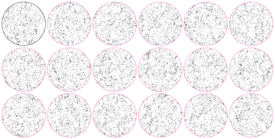
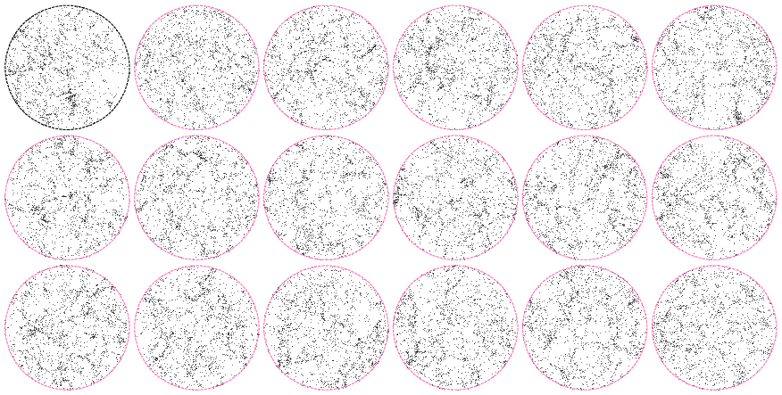
- They select the same kind of region in the sky from both data and simulation (like cutting the same-sized circular slice—called a “cylinder”—from each).
- They include “redshift-space distortions,” which is a technical way of saying they correct for the fact that galaxies also move around inside clusters. This motion can make galaxies look slightly closer or farther along our line-of-sight, a bit like motion blur.
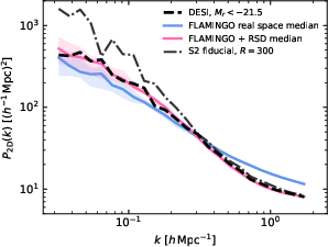
- They measure “how clumpy” things are at different sizes using a tool called a power spectrum. You can think of this like checking whether the map has more big blobs, medium blobs, or tiny blobs of galaxies—similar to how music has bass, mids, and treble.
Most importantly, they carefully compute distances in the correct way. There are two common distance types in astronomy:
- Comoving distance: the “map distance” used to place galaxies in 3D space.
- Luminosity distance: the “brightness-based distance” used to figure out how bright something really is.
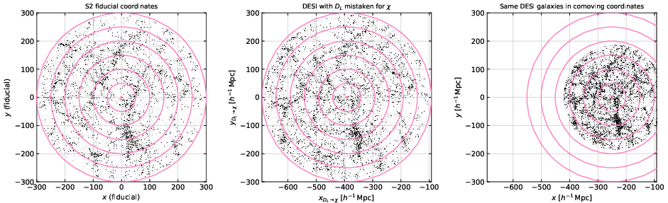
Mixing those up is like confusing miles and kilometers on a map—it stretches the map and creates illusions of huge structures.
What did they find, and why does it matter?
Here are the key results:
- When distances are calculated correctly, the DESI galaxy patterns look normal: The observed galaxy distribution and the simulation look very similar, both by eye and by the power spectrum. In other words, DESI’s map matches what ΛCDM predicts.
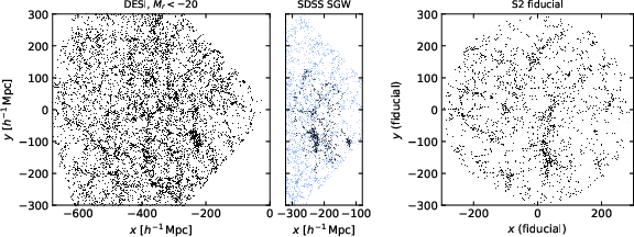
- The earlier claim of an anomaly came from a distance mix-up: The other study treated luminosity distances (in Mpc) as if they were comoving distances (in Mpc). That mistake makes the map look 1.5 to almost 1.8 times larger than it really is, especially for more distant galaxies. It also introduces fake “directional” effects, making the Universe look more uneven than it is.
- Famous known structure, not new physics: The striking feature they saw is the “Sloan Great Wall,” a very well-known large structure. On a properly scaled map, it looks just as it should.
- Motion matters: When you include galaxy motions (redshift-space distortions), the observed and simulated clumpiness match across different sizes. If you ignore this effect, things can look wrongly smoother or bumpier.
Why this matters:
- It supports the cosmological principle: On very large scales, the Universe still looks statistically uniform and the same in all directions.
- It shows how careful you must be with distance definitions and units. A small technical mistake can create big, misleading “discoveries.”
What does this mean for the future?
The big takeaway is reassurance: we don’t need to throw out the standard model of the Universe based on these local galaxy patterns. The results back up the idea that ΛCDM is doing a good job describing large-scale structure. That said, scientists are still testing details of dark energy and other subtle effects with many datasets. This paper reminds us that careful, apples-to-apples comparisons—and the right distances—are essential when mapping the cosmos.
Knowledge Gaps
Knowledge gaps, limitations, and open questions
Below is a focused list of what remains uncertain or unexplored in the paper, framed to guide concrete follow-up work.
- Quantitative audit of the S2 pipeline: Provide a definitive, reproducible demonstration (code and logs) that S2 distances were derived as luminosity distances in Mpc but used as comoving distances in , including re-running the S2 processing with corrected distances and reporting the change in all summary statistics.
- Generalization across DESI tracers: Extend the analysis from BGS to LRG, ELG, and QSO samples and to higher redshifts to test whether conclusions hold across different biases, number densities, and selection functions.
- Full 3D homogeneity and isotropy tests: Move beyond 2D projected slices and windowed to 3D clustering diagnostics (e.g., 3D power-spectrum multipoles, correlation function , BipoSH, Minkowski functionals, genus, fractal dimension ) to directly assess isotropy and the scale of homogeneity.
- Survey mask and selection-function realism: Incorporate the exact DESI angular mask, tiling geometry, completeness, fiber assignment effects, and radial selection function into mock light-cone catalogs; quantify their impact on large-scale power and anisotropy.
- Light-cone mocks and evolution: Use light-cone outputs (rather than single snapshots) that span the observed redshift range (–$0.24$) to include growth and bias evolution along the line of sight and assess their effect on projected clustering.
- Shot-noise treatment and window-function deconvolution: Apply standard shot-noise corrections and/or use estimators that deconvolve the finite-aperture window to ensure large-scale power comparisons are unbiased.
- Redshift-space distortion (RSD) modeling systematics: Test sensitivity to RSD assumptions (e.g., growth rate , galaxy bias, Fingers-of-God damping models) and quantify how RSD uncertainties propagate to the observed large- and small-scale power.
- Galaxy bias calibration: Validate that FLAMINGO galaxies selected by -band luminosity reproduce the DESI BGS clustering bias; if necessary, calibrate with HOD/SHAM approaches and compare hydrodynamic vs. semi-empirical mocks.
- Cosmology dependence: Explore robustness to variations in cosmological parameters (e.g., , , , ) and alternative dark-energy models (CDM), including whether modest shifts affect the consistency with DESI BGS.
- Cosmic variance quantification: Use multiple independent large-volume simulations (different seeds and boxes, e.g., AbacusSummit, Quijote, Uchuu, larger FLAMINGO volumes) to obtain an accurate cosmic variance band; assess whether cylinders drawn from a single box under- or over-estimate variance.
- Cylinder geometry sensitivity: Systematically vary cylinder radius and slab thickness (e.g., –, –) to test how conclusions depend on aperture choices and boundary effects.
- Anisotropy quantification from mis-scaling: Provide a formal estimator (e.g., directional multipoles or BipoSH) showing the magnitude and angular dependence of anisotropy induced by the redshift-dependent scaling error; compare to S2’s reported anisotropy.
- Cross-survey validation: Replicate the analysis in overlapping regions with SDSS DR18 and other spectroscopic surveys to confirm the identification and scale of the Sloan Great Wall and surrounding structures in properly scaled 3D coordinates.
- Completeness and K-correction robustness: Replace the approximate with survey-grade K-corrections and SED-based -terms; produce completeness curves to justify the volume-limited threshold and test sensitivity to magnitude limits.
- Photometric and calibration systematics: Quantify potential impacts of residual extinction, zero-point variations, and color terms in Legacy Surveys photometry on BGS selection and clustering, especially across the chosen angular subregion.
- Statistical significance framework: Complement visual and median-band comparisons with formal hypothesis tests (e.g., p-values, posterior odds, likelihood ratios) for homogeneity/isotropy vs. anisotropy models, explicitly accounting for window functions and covariance.
- Real-space reconstruction cross-check: Attempt RSD inversion or use reconstruction techniques to estimate real-space clustering in the DESI region and compare to real-space simulation slices, isolating RSD contributions.
- Alternative structural statistics: Measure counts-in-cells, void statistics, percolation thresholds, and network/graph measures (e.g., minimum spanning tree metrics) to test large-scale connectivity claims beyond the power spectrum.
- Homogeneity scale measurement: Derive the scale at which (or equivalent homogeneity scale estimators) in the DESI BGS region and compare to predictions, including uncertainty bands and systematics checks.
- Orientation and hemispherical tests: Test for directional asymmetries by rotating the cylinder orientation and scanning different subregions within the DESI footprint to assess robustness against sky geometry and potential dipole-like signals.
- Impact of observer motion assumptions: Evaluate whether the assumption of an observer at rest with respect to the background introduces any bias on the largest modes and, if needed, include the Solar System/CMB dipole in mock RSD.
- Reanalysis of all Sylos Labini datasets: If the mis-scaling affected not only S2 but also other samples (e.g., LRG), perform a comprehensive reanalysis with corrected distances and publish the updated anisotropy measures.
- Boundary and edge effects: Quantify how proximity to the survey footprint edges (e.g., exceeding the footprint) biases mode estimation and clustering, and adopt techniques to mitigate edge-induced anisotropy.
- Reproducibility enhancements: Provide end-to-end scripts to ingest raw DESI catalogs, compute distances, apply selections, and generate all statistics, enabling independent verification and facilitating extensions to other regions/tracers.
Practical Applications
Practical Applications Derived from the Paper
Below is a curated set of actionable applications rooted in the paper’s findings and methods—particularly its demonstration of correct distance scaling, geometry‑matched simulation mocks, redshift‑space distortion (RSD) handling, and windowed power‑spectrum analysis. Items are grouped by deployment horizon and include sector links, potential tools/products, and feasibility notes.
Immediate Applications
- Unit- and Coordinate-Consistency QA for Survey Pipelines
- Sectors: astronomy (observatories, survey consortia), software/data engineering, data governance
- Use cases: Automated checks that detect misapplication of luminosity distance vs. comoving distance; unit-aware transformations; validation that windowing and selection functions are applied consistently.
- Potential tools/products/workflows:
- “CosmoUnitGuard” QA module (Astropy-units–backed validators, schema checks for vs. , Mpc vs. Mpc)
- CI hooks for analysis notebooks/scripts that assert unit integrity before figure/publication generation
- Assumptions/dependencies: Rich metadata and explicit unit tags in catalogs; adoption of Astropy units; team buy-in to enforce QA gates.
- Geometry-Matched Mock Catalogs for Survey Validation and Design
- Sectors: academia (cosmology groups), observatories, HPC/cloud services
- Use cases: Construct “like-for-like” mocks (with RSD and selection) for any sky region to benchmark observed clustering against CDM expectations and quantify cosmic variance.
- Potential tools/products/workflows:
- Modular “GeoMatchMocker” pipeline to extract cylinders/slabs matching survey geometry from public sims (e.g., FLAMINGO)
- Precomputed mock packs for common survey footprints
- Assumptions/dependencies: Access to large simulations (FLAMINGO or equivalents), documented selection functions, basic compute resources.
- RSD-Aware Clustering Analysis
- Sectors: astronomy, scientific software
- Use cases: Routine inclusion of redshift-space distortions in mocks and analyses to avoid false discrepancies; training analysts on visual/quantitative impacts of RSD.
- Potential tools/products/workflows:
- “RSDKit” module to add line-of-sight velocity displacements to mock catalogs; plug-ins for common analysis stacks
- Assumptions/dependencies: Availability of credible peculiar velocities in simulations; validated redshift error models.
- Windowed 2D Power-Spectrum Estimation for Finite Apertures
- Sectors: astronomy; transferable to geoscience, remote sensing, and materials imaging
- Use cases: Comparing observations and simulations without deconvolving complex windows; fast checks of scale-dependent clustering within circular (or survey-specific) windows.
- Potential tools/products/workflows:
- “WindowPS2D” library (FFT-based estimators, aperture-aware binning)
- Assumptions/dependencies: Adequate sampling density; grid and aperture choices tuned to instrument/survey specifics.
- Reproducible Research Templates and Governance
- Sectors: academia, publishers, research policy
- Use cases: End-to-end reproducibility for figures/claims; mandatory code/data release; “verification notebooks” reviewers can run.
- Potential tools/products/workflows:
- GitHub templates that package Astropy/Numpy/Matplotlib code and data snapshots; DOI-minted archives
- Assumptions/dependencies: Open-source dependencies; institutional encouragement or mandates from journals/funders.
- Education and Training Modules on Cosmological Distances and Scale Effects
- Sectors: education (undergrad/grad programs), professional development
- Use cases: Labs demonstrating vs. , unit conversions, RSD, and cosmic variance; case studies preventing “scale-mixing” errors.
- Potential tools/products/workflows:
- Jupyter-based interactive notebooks, small datasets from DESI and FLAMINGO
- Assumptions/dependencies: Stable access to public datasets; curricula bandwidth.
- Visualization Best Practices for Geometry-Consistent Comparisons
- Sectors: science communication, analytics
- Use cases: Standardized figure templates ensuring comparable scales/axes; overlays showing expected RSD and selection effects.
- Potential tools/products/workflows:
- Matplotlib/Plotly presets enforcing axis units and distance conventions; figure audit checklists
- Assumptions/dependencies: Analyst adoption; minimal training.
- Cross-Domain Unit/Scale Checklists for Spatial Analytics
- Sectors: GIS/remote sensing, robotics, finance (spatial risk), energy (geospatial planning)
- Use cases: Prevent “unit-confusion” in coordinate frames (e.g., WGS84 vs. projected), scaling of proxy distances, and window-function misinterpretation.
- Potential tools/products/workflows:
- Sector-specific QA checklists and lints; integration with GIS toolchains (e.g., GDAL plugins)
- Assumptions/dependencies: Domain-specific mapping of cosmology analogs (e.g., “RSD” ↔ motion distortions); willingness to adopt QA steps.
Long-Term Applications
- Simulation-Backed Anomaly Classifiers (Simulation-Based Inference)
- Sectors: astronomy, ML/AI for science
- Use cases: Automatically flag whether observed “anomalies” exceed cosmic variance given survey geometry and selection, using ensembles of mocks.
- Potential tools/products/workflows:
- “CosmoSBI” pipeline integrating fast emulators of clustering statistics with window/RSD modeling
- Assumptions/dependencies: Large, diverse simulation suites; compute budgets; careful treatment of selection systematics.
- Unit-Aware, Type-Safe Cosmological Coordinate Framework
- Sectors: scientific software, data infrastructure
- Use cases: Strong typing of , , , and Mpc vs. Mpc; compile-/runtime checks that prevent misuse in pipelines.
- Potential tools/products/workflows:
- “cosmo-coords” library built atop Astropy units/pydantic/typing; schema enforcement in HDF5/Parquet
- Assumptions/dependencies: Broad ecosystem adoption; backwards-compatible data model evolution.
- Real-Time Survey Digital Twins
- Sectors: observatories, HPC/cloud providers
- Use cases: On-the-fly geometry-matched mocks during survey operations to validate emerging features; dynamic assessment of cosmic variance and systematics.
- Potential tools/products/workflows:
- “SurveyTwin” service orchestrating simulation slices, RSD, and windowed stats in near-real-time
- Assumptions/dependencies: Streamlined access to simulation data; scalable cloud/HPC; robust, fast selection-function modeling.
- Generalization of Windowed Spectral Methods to Other Sensing Domains
- Sectors: earth observation (SAR, altimetry), healthcare (medical imaging), materials science (DVC/DIC)
- Use cases: Aperture/window-aware power analysis to avoid over/underestimating structure in bounded fields-of-view.
- Potential tools/products/workflows:
- Domain-adapted “WindowPS2D/3D” toolkits with instrument-specific windows
- Assumptions/dependencies: Domain-specific calibration; validation against physical benchmarks.
- RSD-Analogue Corrections in Motion-Sensing Systems
- Sectors: robotics/autonomous vehicles, defense (radar), industrial sensing
- Use cases: Correcting motion-induced distortions (Doppler/range-rate effects) in point clouds; improving spatial statistics for mapping/localization.
- Potential tools/products/workflows:
- “RSD-Analog” modules for LiDAR/radar pipelines (line-of-sight velocity modeling and correction)
- Assumptions/dependencies: Accurate sensor motion/velocity models; synchronization with IMU/GNSS; robust calibration.
- Policy and Publishing Guidelines for Anomaly Claims and Reproducibility
- Sectors: research governance, journals, funding agencies
- Use cases: Pre-submission checks requiring unit-validated code, simulation-backed baselines, and window-aware statistics.
- Potential tools/products/workflows:
- Standardized checklists and reproducibility badges; reviewer-run verification notebooks
- Assumptions/dependencies: Community and publisher buy-in; guidance for exceptions.
- Curricular Standards and Credentialing for “Data Unit Literacy”
- Sectors: education, professional certification
- Use cases: Formal training and micro-credentials in units/coordinates for data-intensive sciences.
- Potential tools/products/workflows:
- MOOCs, certification exams, and institutional modules based on the paper’s case study
- Assumptions/dependencies: Departmental adoption; alignment with accreditation bodies.
- Cloud Marketplaces for Prebuilt Cosmological Mock Catalogs
- Sectors: cloud/data marketplaces, observatories
- Use cases: Datasets-as-a-service offering geometry-matched mocks for common surveys (DESI, Euclid, LSST) with RSD and selection functions.
- Potential tools/products/workflows:
- Curated “MockPacks” with versioned metadata and unit-safe schemas
- Assumptions/dependencies: Licensing/IP constraints; sustainable funding models.
- Physics-Consistent Anomaly Detection Frameworks Beyond Astronomy
- Sectors: climate/earth systems, finance (market microstructure), network science
- Use cases: Benchmark anomalies against physics-/mechanism-based simulations while honoring window/selection effects.
- Potential tools/products/workflows:
- Cross-domain SBI frameworks with “window-aware” statistics and typed units
- Assumptions/dependencies: Existence of credible simulators; mapping of observational windows and distortions to domain.
Summary Note
The paper’s central contribution—showing that correct distance scaling and RSD-aware, geometry-matched comparisons reconcile observations with CDM—translates directly into robust QA, analysis, and reproducibility practices that are deployable now. Longer-term, automation, unit-safe frameworks, and digital twins can institutionalize these safeguards across astronomy and inspire analogous safeguards in other data‑intensive fields.
Glossary
- AGN feedback: Energy and momentum injected into surrounding gas by an active galactic nucleus, affecting galaxy evolution and heating/expelling gas. Example: "massive black holes and thermal AGN feedback."
- a posteriori feature selection: Choosing patterns or statistics after inspecting the data, which can inflate apparent significance. Example: "a posteriori feature selection and look-elsewhere effects"
- absolute magnitude: An intrinsic measure of an object’s brightness defined as the apparent magnitude at a standard distance of 10 parsecs. Example: "The absolute magnitude used for the selection is then"
- Baryon Acoustic Oscillations (BAO): Regular, periodic fluctuations in the density of the visible baryonic matter of the universe, used as a standard ruler. Example: "combining DESI BAO measurements with CMB and supernova data"
- cold dark matter (CDM): A form of dark matter consisting of slow-moving particles that interact gravitationally, forming structure hierarchically. Example: "Such features are also a natural outcome of cold-dark-matter simulations"
- comoving distance: A distance measure that accounts for the expansion of the universe, keeping object separations fixed in comoving coordinates. Example: "comoving distances are computed directly from the published, spectroscopic redshifts."
- cosmic microwave background (CMB): Relic radiation from the early universe, providing a snapshot of conditions ~380,000 years after the Big Bang. Example: "combining DESI BAO measurements with CMB and supernova data"
- cosmic variance: Statistical uncertainty arising because we observe only one realization of the universe’s large-scale structure. Example: "The large-scale modes show considerable cosmic variance."
- cosmic web: The large-scale structure of the universe composed of interconnected filaments, sheets, clusters, and voids. Example: "modern observations reveal a complex cosmic web of voids, filaments, clusters and superclusters"
- cosmological principle: The assumption that the universe is statistically homogeneous and isotropic on large scales. Example: "The cosmological principle, which states that the Universe is statistically homogeneous and isotropic on sufficiently large scales, is a foundational assumption of the standard cosmological model."
- D3A cosmology: A specific cosmological parameter set used for distance calculations and simulations in the paper. Example: "Throughout this work, the D3A cosmology is adopted, with , , , , , , and ."
- distance modulus: The difference between an object’s apparent and absolute magnitudes, used to compute distances from photometry. Example: "The physical luminosity distance, , can be inferred from the distance modulus,"
- Friedmann--Lemaître--Robertson--Walker (FLRW) framework: The standard cosmological model assuming a homogeneous and isotropic universe, described by the FLRW metric. Example: "in the broader Friedmann--Lema^itre--Robertson--Walker framework."
- FLAMINGO (cosmological hydrodynamic simulation): A large-scale simulation including gravity, gas dynamics, and galaxy formation physics used to generate mock catalogs. Example: "the FLAMINGO cosmological hydrodynamic simulation"
- geometry-matched mocks: Synthetic data constructed to match the observational geometry and selection, enabling fair comparisons. Example: "geometry-matched mocks based on CDM simulations."
- gigaparsec (Gpc): A distance unit equal to one billion parsecs (~3.26 billion light years), used for very large-scale structures. Example: "extending to gigaparsec scales"
- HBT-HERONS: A specific halo and galaxy identification algorithm/tool used to find bound structures in simulations. Example: "Haloes and galaxies are identified with HBT-HERONS"
- hierarchical structure formation: The theoretical picture in which small structures form first and merge into larger ones over time. Example: "The standard paradigm of hierarchical structure formation predicts a Universe that is strongly inhomogeneous on the scales of galaxies and galaxy clusters, but statistically homogeneous and isotropic on sufficiently large scales"
- (Hubble-scaled comoving units): A distance unit rescaled by the dimensionless Hubble parameter , commonly used in cosmology. Example: "as comoving distances in units of ."
- K-correction: A correction applied to observed magnitudes to account for redshifted spectra, transforming them to rest-frame bands. Example: "applying the low-redshift -band -correction"
- CDM (Lambda-CDM): The standard cosmological model including cold dark matter and a cosmological constant . Example: "performed in the standard CDM paradigm."
- look-elsewhere effect: The increased chance of finding apparently significant signals when multiple comparisons or searches are conducted. Example: "look-elsewhere effects"
- luminosity distance: A distance measure derived from observed brightness, relating flux to intrinsic luminosity in an expanding universe. Example: "The physical luminosity distance, , can be inferred from the distance modulus,"
- mock galaxy catalogue: A simulated galaxy dataset built to mimic observational samples for testing analyses and models. Example: "geometry-matched mock galaxy catalogues are constructed based on the FLAMINGO cosmological hydrodynamic simulation"
- peculiar velocity: An object’s velocity relative to the uniform Hubble expansion, causing redshift-space distortions. Example: "the line-of-sight peculiar velocity is"
- periodic cube (simulation box): A computational volume with periodic boundary conditions used in cosmological simulations. Example: "evolves a periodic cube of side length "
- power spectrum: A statistic quantifying clustering strength as a function of scale by decomposing the density field into Fourier modes. Example: "Power spectra comparison between DESI, FLAMINGO, and S2."
- redshift-space distortions (RSD): Apparent anisotropies in galaxy positions due to line-of-sight velocities affecting observed redshifts. Example: "redshift-space distortions are added according to the peculiar velocity data."
- shot noise: Random fluctuations from the discrete sampling of galaxies, impacting small-scale clustering measurements. Example: "The small-scale behaviour is affected by both redshift-space distortions and shot noise."
- Sloan Great Wall: A prominent, large-scale structure (supercluster complex) in the nearby universe. Example: "the ``Sloan Great Wall", a prominent structure in the Local Universe"
- statistical homogeneity and isotropy: The property that, on large scales, the universe’s statistical properties do not depend on location or direction. Example: "statistically homogeneous and isotropic on sufficiently large scales"
- volume-limited sample: A galaxy sample defined so all objects above a luminosity threshold are included out to a fixed distance, avoiding selection bias. Example: "Using a volume-limited sample from the bright galaxy catalogue of DESI DR1"
- window function: The effect of a finite survey geometry or aperture on measured statistics, filtering modes in Fourier space. Example: "the finite circular aperture has a non-trivial window function."
- windowed two-dimensional power spectra: Power spectra measured within a finite 2D aperture, incorporating the survey’s window function. Example: "windowed two-dimensional power spectra in circular apertures."