Theory and Applications of Convolution-Based short time offset linear canonical transform

Abstract: In this paper, we introduce a convolution based short time offset linear canonical transform (STOLCT) and investigate its fundamental mathematical properties. Specifically, we establish its continuity, orthogonality relations, inversion formulas, range theorem, and convolution theorem. We further explore several important applications of STOLCT, including the Poisson summation formula, the Paley Wiener criterion, and a sampling theorem. In addition, numerical simulations and graphical analyses are presented to compare signal reconstruction performance under different scenarios. A comparative study between STOLCT and STLCT is conducted with respect to their reconstruction formulas, demonstrating the effectiveness and potential advantages of the proposed transform.

• The paper introduces STOLCT, a convolution-based extension that allows localized analysis of OLCT for non-stationary, chirp-like signals.
• It establishes fundamental properties including continuity, orthogonality preserving energy, and an explicit inversion formula for exact signal reconstruction.
• Numerical experiments demonstrate STOLCT’s superior performance with reduced reconstruction errors compared to traditional STLCT methods.

Convolution-Based Short Time Offset Linear Canonical Transform: Theory and Applications

Motivation and Transform Construction

The offset linear canonical transform (OLCT) generalizes the classical Fourier and linear canonical transforms by introducing additional parameters for time and frequency shifts, enabling more effective representation of non-stationary signals, especially those exhibiting chirp-like and quadratic phase characteristics. However, OLCT, with its global kernel, lacks local time-frequency analysis capability. This paper introduces the convolution-based short time offset linear canonical transform (STOLCT), which achieves localized OLCT-frequency analysis with temporal windows via convolution in the OLCT domain.

STOLCT's formulation leverages an analyzing function modulated by OLCT's kernel. The transform is defined for signals $f \in L^2(\mathbb{R})$ with window $g \in L^2(\mathbb{R})$:

$$\mathcal{O}_{g_w}[f](u, \eta) = \frac{1}{\sqrt{2\pi ib}} \int_{\mathbb{R}} f(x) \overline{g(x-u)} e^{\frac{-iax}{b}(u-x) + \frac{i}{2b} du_0^2 - i \eta x} dx$$

This construction inherits OLCT's flexibility, allowing direct analysis and reconstruction of signals with arbitrary offsets without explicit compensation matrices.

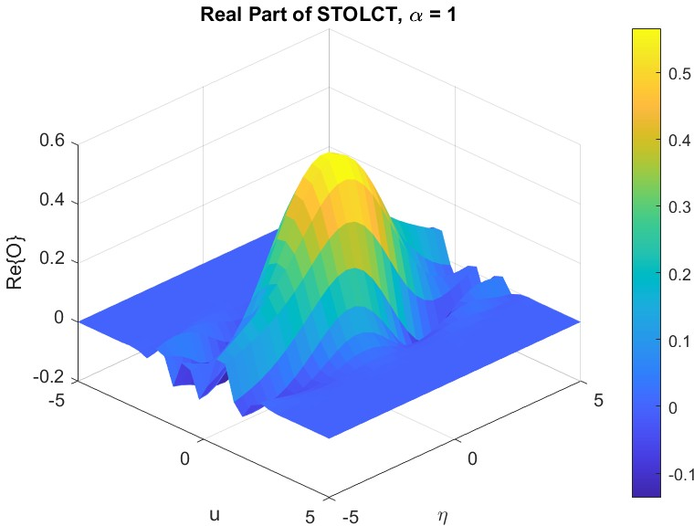
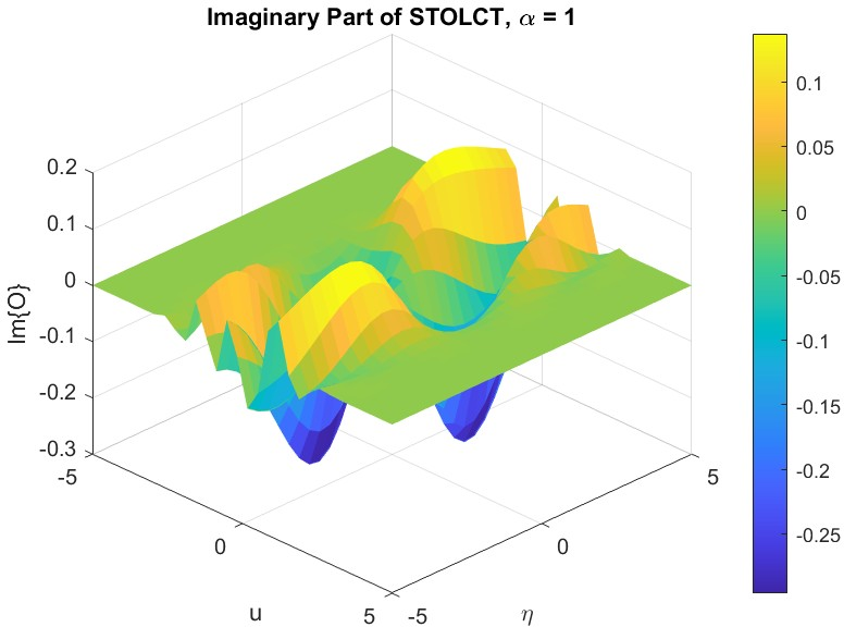
Figure 1: Real and Imaginary components for $\alpha=1$ with Gaussian signal and rectangular window, illustrating the complex nature of STOLCT outputs for moderate decay.

Fundamental Properties: Continuity, Orthogonality, Inversion

The paper rigorously establishes several key mathematical properties of STOLCT:

• Continuity: STOLCT is continuous in both its time and frequency parameters, as shown via direct limit analysis in the transform's integral representation.
• Orthogonality: The inner product structure is preserved; the energy of the transform equals the product of signal and window energies:

$$\int_{\mathbb{R}^2} |\mathcal{O}_{g_w}[f](u, \tau)|^2 du d\tau = ||f||^2 ||g||^2$$

This extends the Plancherel property to the OLCT domain and confirms energy conservation.

• Inversion Formula: Signals can be exactly reconstructed from their STOLCT via an explicit integral formula involving the analyzing function:

$$f(t) = \frac{1}{\overline{\sqrt{2\pi ib} \langle g_2, g_1 \rangle}} \int_{\mathbb{R}^2} \mathcal{O}_{g_w}[f](u, \tau) g^M_{2,u,\tau}(t) du d\tau$$

where $g^M_{2,u,\tau}(t)$ is the OLCT-parametrized analyzing function.

Numerical Characterization and Parameter Sensitivity

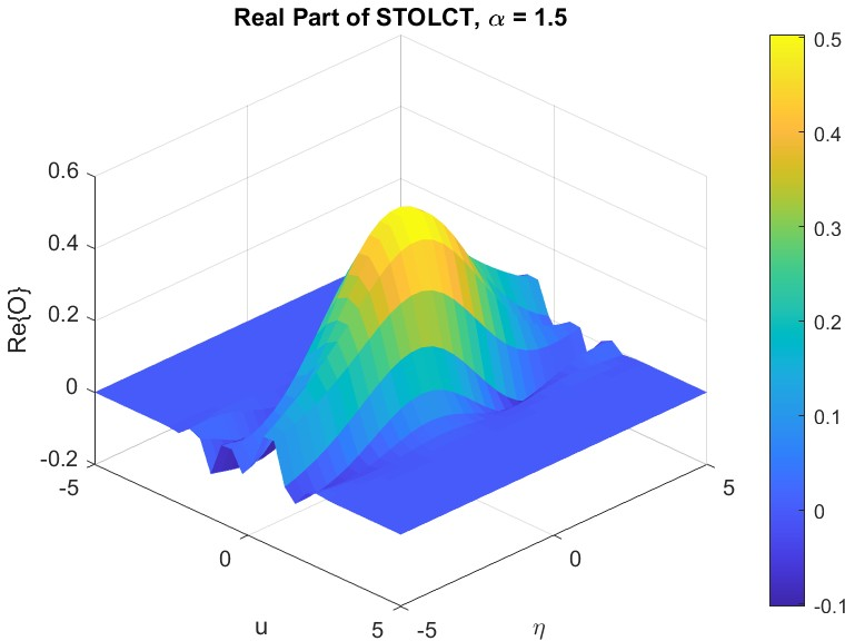
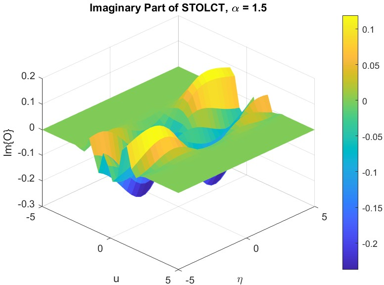
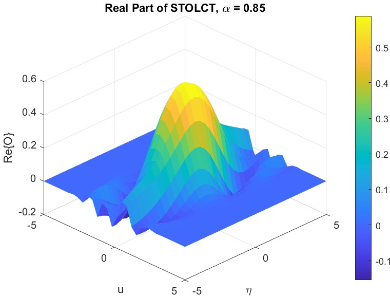
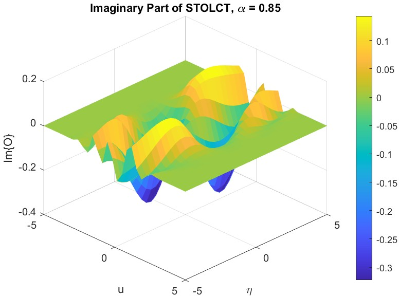
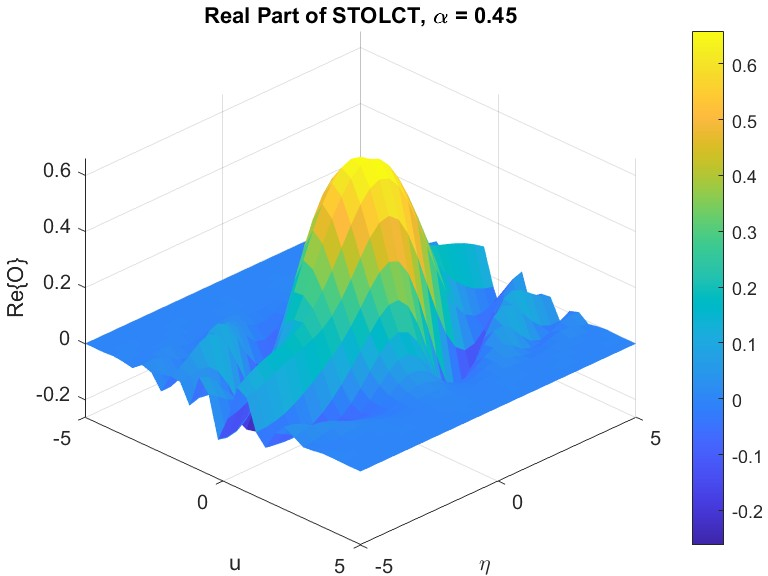
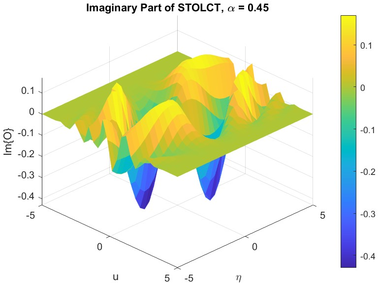
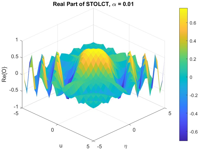
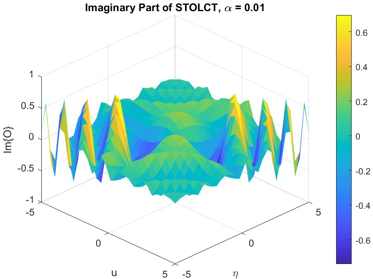
Numerical simulations for Gaussian signals and various window functions elucidate STOLCT's sensitivity to decay parameter $\alpha$ and bandlimited parameter $\eta$. As $\alpha$ decreases, the real and imaginary components of the STOLCT output converge, indicating a balanced complex profile. The transform remains stable and robust across parameter ranges, enabling accurate localized analysis of both theoretical and practical signals.

Figure 2: Real and Imaginary components for $g \in L^2(\mathbb{R})$0, demonstrating the signal's localization and complex structure variation as $g \in L^2(\mathbb{R})$1 increases.

Figure 3: Real and Imaginary components for $g \in L^2(\mathbb{R})$2, showing further complex evolution.

Figure 4: Real and Imaginary components for $g \in L^2(\mathbb{R})$3, highlighting the monotonic increase in real and imaginary values as decay decreases.

Figure 5: Real and Imaginary components for $g \in L^2(\mathbb{R})$4, illustrating nearly equal real/imaginary values for very slow decay.

Convolution Theorem and Range Characterization

The convolution theorem holds in the STOLCT domain, allowing signal products to be analyzed via their STOLCTs:

$g \in L^2(\mathbb{R})$5

This is complemented by a range characterization theorem proving that a function $g \in L^2(\mathbb{R})$6 is a valid STOLCT if and only if it satisfies a reproducing kernel integral constraint.

Applications: Summation, Criterion, Sampling

Poisson Summation Formula

STOLCT supports a generalized Poisson summation formula. Time-domain sampling and transform-domain analysis remain connected, extending classical Fourier and OLCT-domain formulas. The infinite sum of time samples of a signal under OLCT convolution yields an equivalent sum of STOLCT coefficients, facilitating analysis and synthesis in both domains.

Paley–Wiener Criterion

STOLCT accommodates the Paley–Wiener criterion for transform-domain bandlimited signals. The criterion is extended:

$g \in L^2(\mathbb{R})$7

ensuring precise control over analytic signal behavior and system stability in the OLCT context.

Sampling Theorem

A Shannon-type sampling theorem is proven for STOLCT, allowing exact signal reconstruction for $g \in L^2(\mathbb{R})$8-bandlimited signals:

$g \in L^2(\mathbb{R})$9

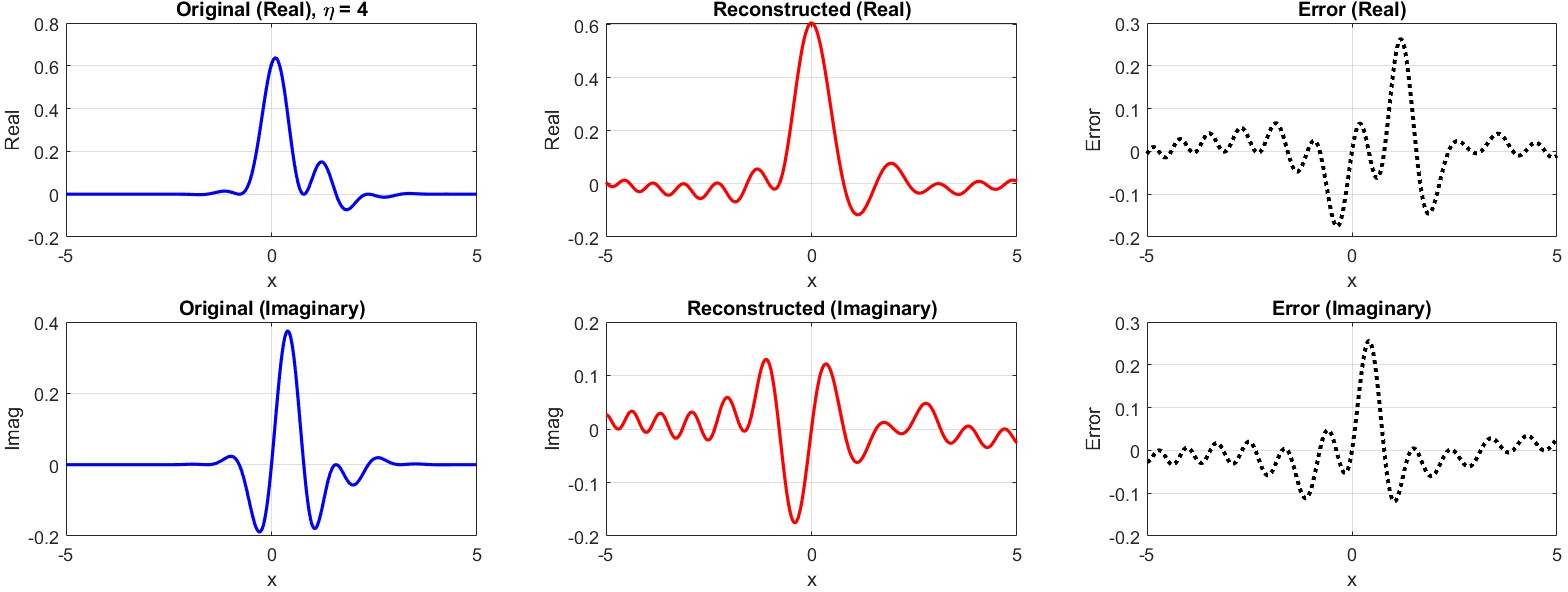
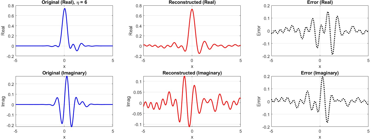
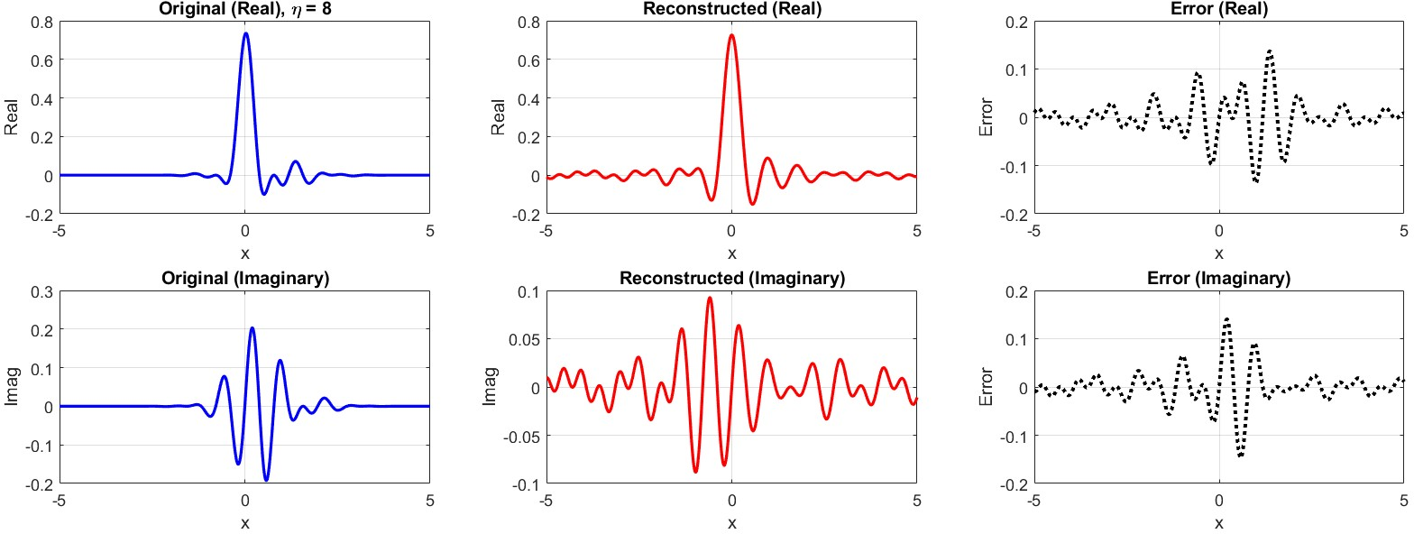
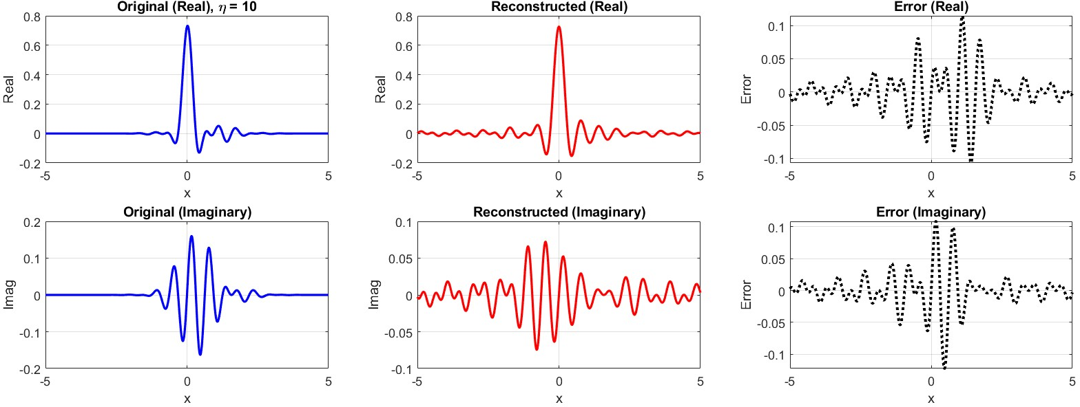
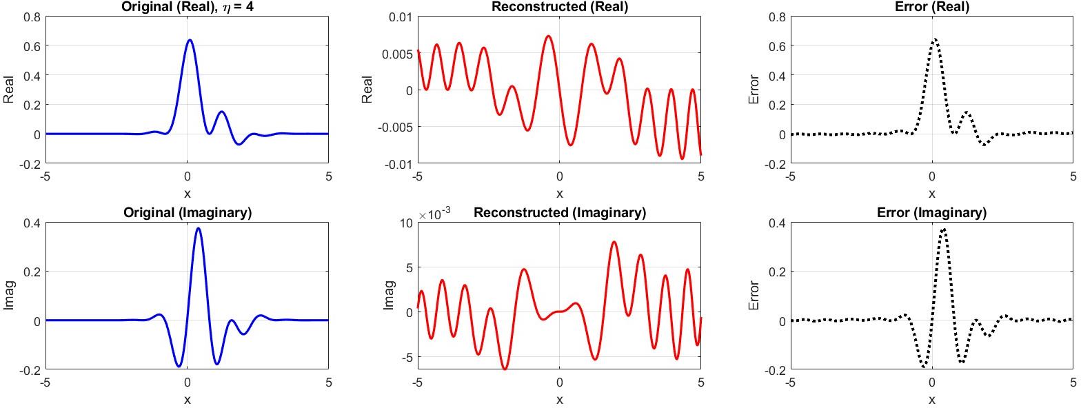
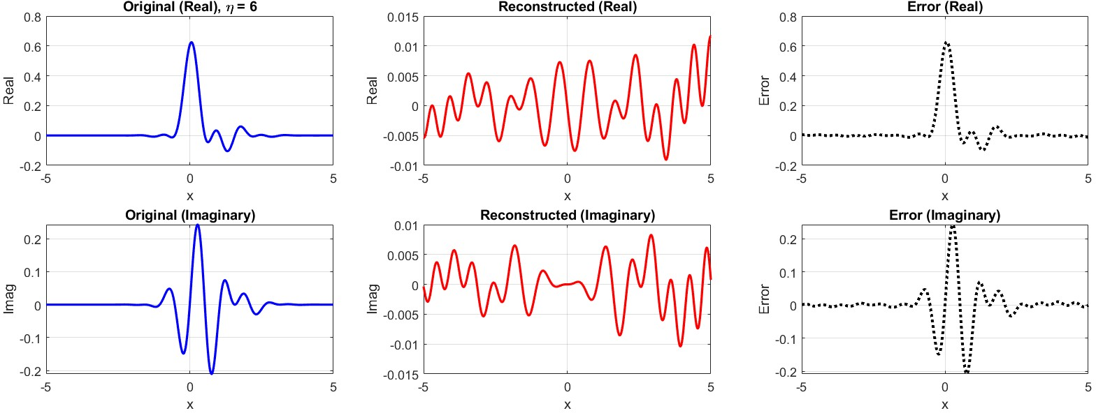
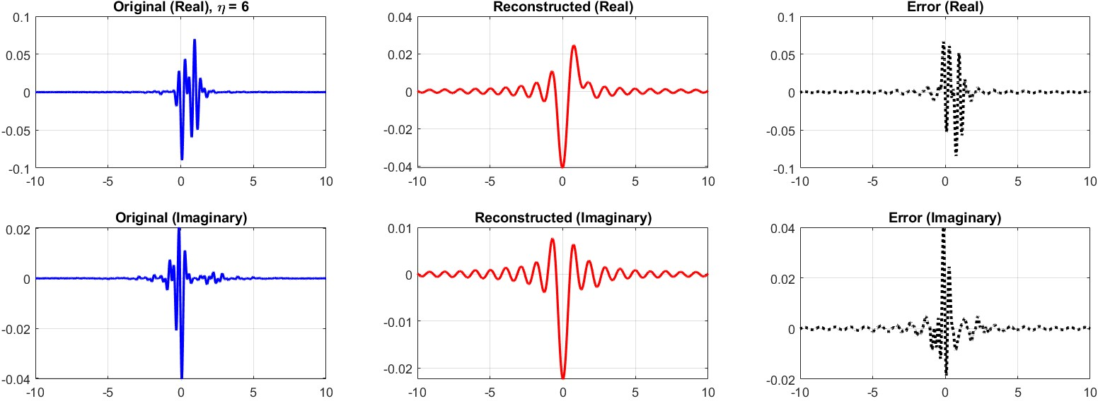
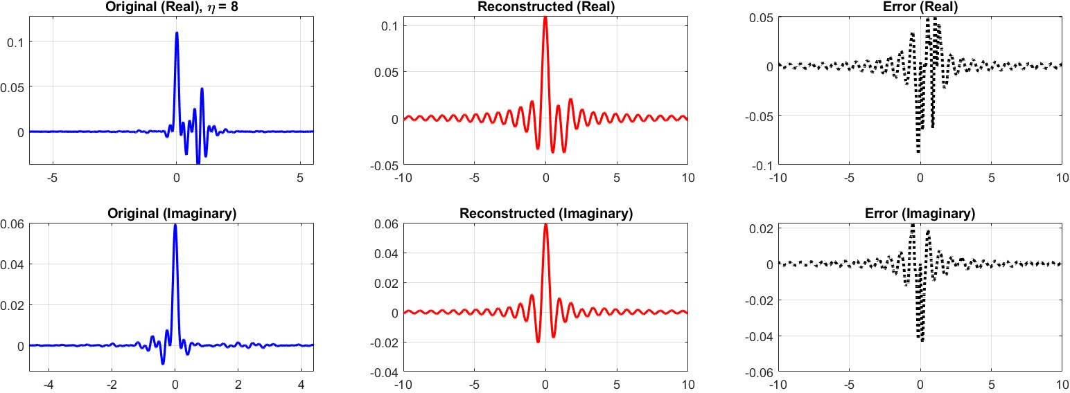
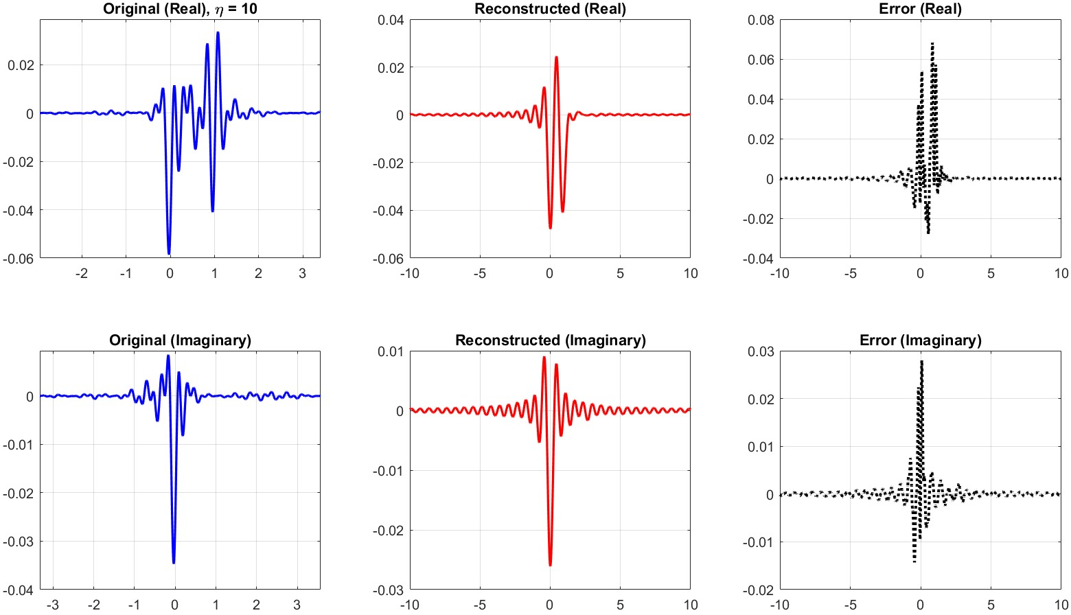
Numerical experiments validate the theoretical reconstruction, with error decaying rapidly as $$\mathcal{O}_{g_w}[f](u, \eta) = \frac{1}{\sqrt{2\pi ib}} \int_{\mathbb{R}} f(x) \overline{g(x-u)} e^{\frac{-iax}{b}(u-x) + \frac{i}{2b} du_0^2 - i \eta x} dx$$0 increases.

Figure 6: Real and Imaginary components of STOLCT reconstruction for $$\mathcal{O}_{g_w}[f](u, \eta) = \frac{1}{\sqrt{2\pi ib}} \int_{\mathbb{R}} f(x) \overline{g(x-u)} e^{\frac{-iax}{b}(u-x) + \frac{i}{2b} du_0^2 - i \eta x} dx$$1 with sinc and Gaussian window, showing high-fidelity output.

Figure 7: Real and imaginary reconstruction errors for STOLCT at $$\mathcal{O}_{g_w}[f](u, \eta) = \frac{1}{\sqrt{2\pi ib}} \int_{\mathbb{R}} f(x) \overline{g(x-u)} e^{\frac{-iax}{b}(u-x) + \frac{i}{2b} du_0^2 - i \eta x} dx$$2, quantifying performance.

Figure 8: Real and imaginary reconstruction errors for STOLCT at $$\mathcal{O}_{g_w}[f](u, \eta) = \frac{1}{\sqrt{2\pi ib}} \int_{\mathbb{R}} f(x) \overline{g(x-u)} e^{\frac{-iax}{b}(u-x) + \frac{i}{2b} du_0^2 - i \eta x} dx$$3.

Figure 9: Real and imaginary reconstruction errors for STOLCT at $$\mathcal{O}_{g_w}[f](u, \eta) = \frac{1}{\sqrt{2\pi ib}} \int_{\mathbb{R}} f(x) \overline{g(x-u)} e^{\frac{-iax}{b}(u-x) + \frac{i}{2b} du_0^2 - i \eta x} dx$$4.

Figure 10: Real and imaginary reconstruction errors for STOLCT at $$\mathcal{O}_{g_w}[f](u, \eta) = \frac{1}{\sqrt{2\pi ib}} \int_{\mathbb{R}} f(x) \overline{g(x-u)} e^{\frac{-iax}{b}(u-x) + \frac{i}{2b} du_0^2 - i \eta x} dx$$5, displaying minimal error at high bandwidth.

Comparative Study: STOLCT vs STLCT

Direct comparison between STOLCT and STLCT sampling methods reveals lower reconstruction errors for STOLCT across all bandwidths. Empirical error analysis confirms STOLCT's superiority, especially at large $$\mathcal{O}_{g_w}[f](u, \eta) = \frac{1}{\sqrt{2\pi ib}} \int_{\mathbb{R}} f(x) \overline{g(x-u)} e^{\frac{-iax}{b}(u-x) + \frac{i}{2b} du_0^2 - i \eta x} dx$$6 values, attributable to offset-parameter flexibility.

Figure 11: STLCT reconstruction error for $$\mathcal{O}_{g_w}[f](u, \eta) = \frac{1}{\sqrt{2\pi ib}} \int_{\mathbb{R}} f(x) \overline{g(x-u)} e^{\frac{-iax}{b}(u-x) + \frac{i}{2b} du_0^2 - i \eta x} dx$$7, illustrating performance gap.

Figure 12: STLCT reconstruction error for $$\mathcal{O}_{g_w}[f](u, \eta) = \frac{1}{\sqrt{2\pi ib}} \int_{\mathbb{R}} f(x) \overline{g(x-u)} e^{\frac{-iax}{b}(u-x) + \frac{i}{2b} du_0^2 - i \eta x} dx$$8.

Figure 13: STLCT reconstruction error for $$\mathcal{O}_{g_w}[f](u, \eta) = \frac{1}{\sqrt{2\pi ib}} \int_{\mathbb{R}} f(x) \overline{g(x-u)} e^{\frac{-iax}{b}(u-x) + \frac{i}{2b} du_0^2 - i \eta x} dx$$9.

Figure 14: STLCT reconstruction error for $\alpha=1$0.

Exact Bandlimited Signal Experiments

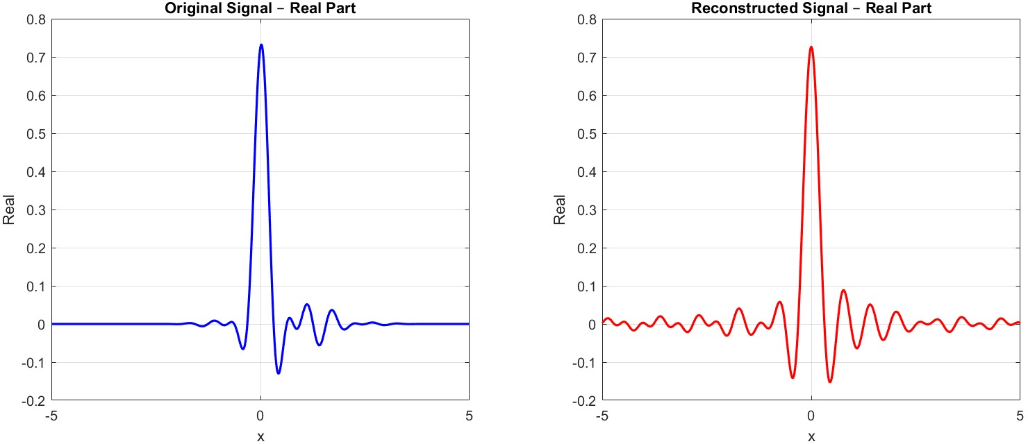
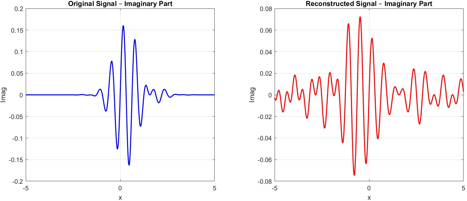
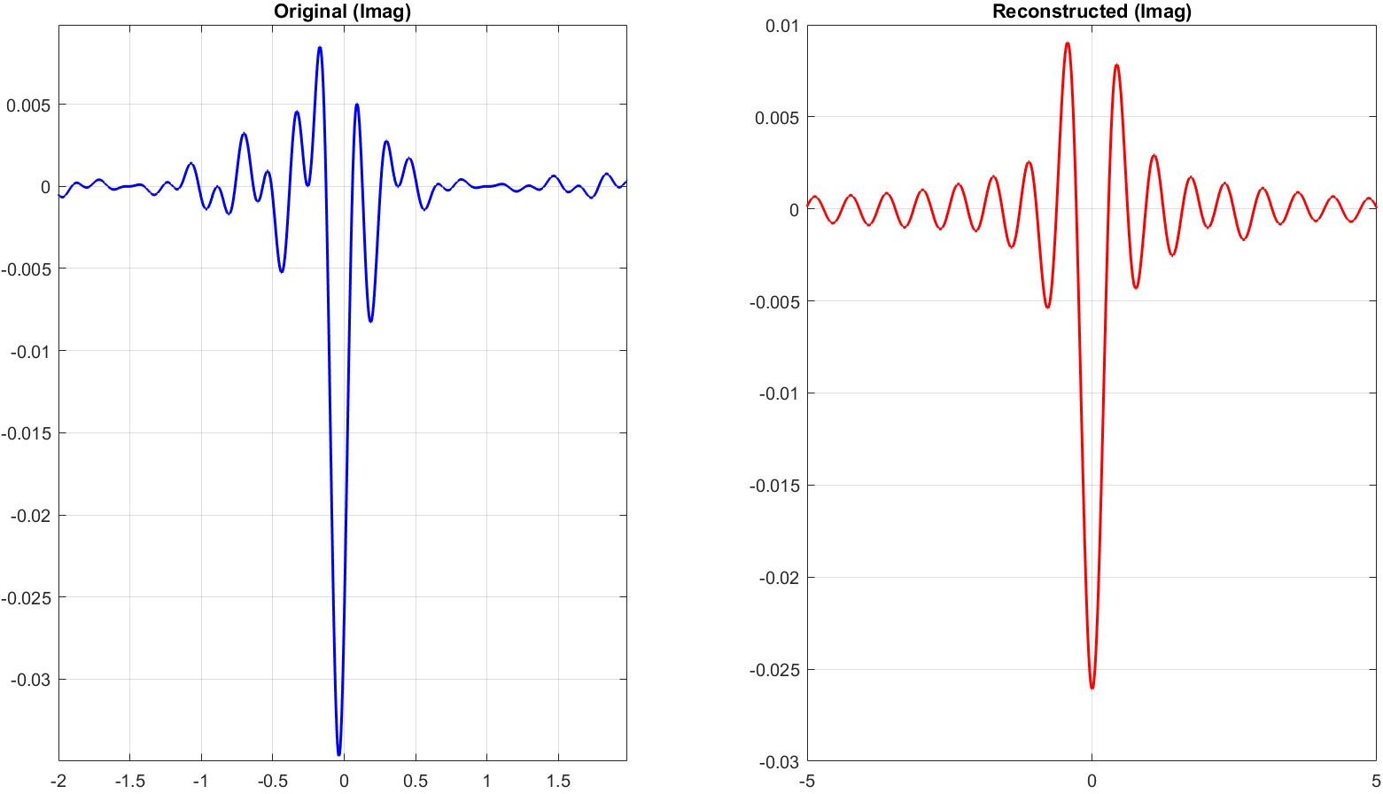
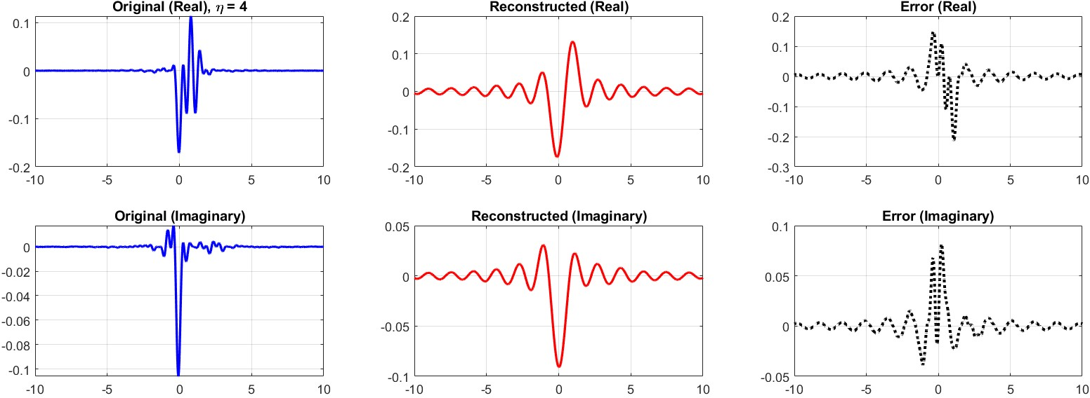
Experiments with strictly bandlimited signals (sinc signals) and windows confirm theoretical exactness of STOLCT-based reconstruction, with errors attributable solely to numerical truncation.

Figure 15: Original versus reconstructed real part for bandlimited signal, $\alpha=1$1.

Figure 16: Original versus reconstructed imaginary part for bandlimited signal, $\alpha=1$2.

Figure 17: Reconstruction error for STOLCT at $\alpha=1$3, showing very low error.

Figure 18: Reconstruction error for STOLCT at $\alpha=1$4.

Figure 19: Reconstruction error for STOLCT at $\alpha=1$5.

Figure 20: Reconstruction error for STOLCT at $\alpha=1$6, indicating improved accuracy.

Implications and Future Directions

The convolution-based STOLCT offers both theoretical and practical advantages for non-stationary, chirp-like signal analysis. Its offset and window parameters provide analytical flexibility suitable for modern signal processing, communication, and optical systems. The transform's mathematical structure enables stable, energy-preserving, and invertible analysis with direct sampling-theoretic reconstruction.

From an AI perspective, STOLCT's ability to capture localized, non-stationary phenomena can benefit neural architectures for time-series and signal interpretation, including hybrid models integrating deep learning with canonical transforms. Future research might address:

• Integration of STOLCT in deep learning pipelines for adaptive, robust feature extraction.
• Parameter optimization for OLCT kernels in automatic signal analysis systems.
• Generalization to higher dimensions and non-Euclidean domains for image and multi-modal data.

Conclusion

This paper introduces the convolution-based STOLCT, rigorously establishing its theoretical properties and demonstrating its advantages through precise comparative analyses and numerical experiments. The transform advances time-frequency analysis for non-stationary signals, supports exact reconstruction, and exhibits lower empirical error compared to related transforms. Its potential for practical deployment in signal processing and AI-driven analysis frameworks is substantial (2606.14102).