Effective Dimensionality as an Operator Invariant for Physics-Preserving Constraint Adaptation in Physics-Informed Neural Networks

Abstract: Physics-Informed Neural Networks inherently suffer from task interference because they rely on a shared parameter space to satisfy both governing differential equations and boundary conditions. We analyze this structural conflict using the Fisher Information Matrix to quantify the effective degrees of freedom ($d_{eff}$) in a physics-constrained model. Unlike the classical $d_{eff}$ which measures how many parameter directions are informed by data against a statistical prior, our $d_{eff}$ measures the dimension of the parameter directions unconstrained by the differential operator. For operators with finite-dimensional kernel, we show that $d_{eff}$ converges to the kernel dimension exactly, independent of network width, depth, or activation function, recasting it from a fit diagnostic into a structural invariant of the underlying continuous operator. For operators with infinite-dimensional kernel, $d_{eff}$ instead measures the network's finite-dimensional representational bandwidth for that kernel rather than recovering an integer invariant. Importantly, $d_{eff}$ also serves as an a priori structural diagnostic. Driving $d_{eff}$ of a well-posed problem to zero certifies that the physics and boundary constraints have absorbed the network's free directions. Building on this characterization, we introduce subspace projection strategies for boundary adaptation. Rather than retraining from scratch, we project parameter updates into the null space of the pre-trained physics operator so that new boundary conditions are satisfied without disturbing the learned physics. Gradient-based fine-tuning can match or exceed this but needs more wall-clock time and tuning, whereas subspace projection delivers near-equivalent quality in seconds to minutes. We validate on linear and nonlinear operators, demonstrating accurate adaptation to initial and boundary shifts and unencountered constraint types.

• The paper introduces effective dimensionality, derived from the Fisher Information Matrix, as a diagnostic tool that quantifies the unconstrained parameter directions in PINNs.
• It develops a null-space projection strategy for boundary adaptation that preserves the learned physics and accelerates convergence compared to traditional gradient-based fine-tuning.
• Empirical results validate that effective dimensionality remains invariant across architectures, accurately matching analytical kernel dimensions in diverse ODE, PDE, and nonlinear model environments.

Effective Dimensionality as an Operator Invariant for Physics-Preserving Constraint Adaptation in PINNs

Introduction and Motivation

Physics-Informed Neural Networks (PINNs) integrate governing differential equations (DEs) and boundary conditions (BCs) within neural network training, leveraging deep learning for scientific modeling. However, the simultaneous enforcement of operator constraints and BCs results in task interference: competing objectives impose conflicting demands on the shared parameter space, often leading to loss ill-conditioning and fragile convergence. Addressing such structural conflicts necessitates quantitative diagnostics and principled adaptation strategies, particularly for real-world deployment where boundary conditions change frequently.

This paper proposes a Fisher Information Matrix (FIM)-based measure, $d_{\text{eff}}$, defining the effective degrees of freedom in PINNs as the dimensionality of parameter directions unconstrained by the physics operator. For operators with finite-dimensional kernels, $d_{\text{eff}}$ converges exactly to the kernel dimension, invariant to network width, depth, or activation. This reframes effective dimensionality from a fit diagnostic to an operator structural invariant, enabling a priori diagnostics and novel adaptation protocols.

Mathematical Formulation of Effective Dimensionality

The effective degrees of freedom $d_{\text{eff}}$ are derived from an information-geometric analysis of the network parameter space. Classical data-driven $d_{\text{eff}}$ measures the number of directions informed by observational data against a statistical prior. In the physics-informed regime, the constraint matrix encodes an operator with a kernel of known dimension, and the trace formula computes the directions the operator leaves unconstrained:

$$d_{\text{eff}} = \operatorname{tr}\left( Q M^{+} Q M^{+} \right)$$

with $M = Q + \lambda_p H_p + \lambda_b H_b$, where $Q$ is the FIM, $H_p$ and $H_b$ are the Hessians from spatial (PDE) and boundary constraints respectively, and $\lambda_p$, $d_{\text{eff}}$0 are penalty weights. As $d_{\text{eff}}$1 and $d_{\text{eff}}$2 (deterministic PINN regime), $d_{\text{eff}}$3 measures the operator's unconstrained directions—the kernel dimension.

The dual-space NTK reformulation—projecting via the empirical Neural Tangent Kernel—makes $d_{\text{eff}}$4 computation tractable for large networks by substituting expensive parameter-space pseudoinverses with function-space projections.

Invariance and Structural Diagnostics

Systematic experiments demonstrate that $d_{\text{eff}}$5 converges precisely to the analytical kernel dimension for a range of ODEs and PDEs, independent of network architecture (width, depth, activation, residual connections):

• Linear ODEs: For an $d_{\text{eff}}$6-th order ODE, $d_{\text{eff}}$7 across all tested architectures.
• Bessel Operator: $d_{\text{eff}}$8 reflecting the two-dimensional kernel of $d_{\text{eff}}$9.
• Nonlinear Operators: For second-order nonlinear PDEs with known kernel properties, $d_{\text{eff}}$0 remains invariant and matches expected analytical values.

This invariance enables $d_{\text{eff}}$1 to serve as a structural diagnostic. In under-resolved regimes, $d_{\text{eff}}$2 saturates at the collocation-point rank, revealing when the training is structurally under-constrained even if the residual loss vanishes. As grid density increases, $d_{\text{eff}}$3 and the predicted PINN solution converge to the true solution manifold.

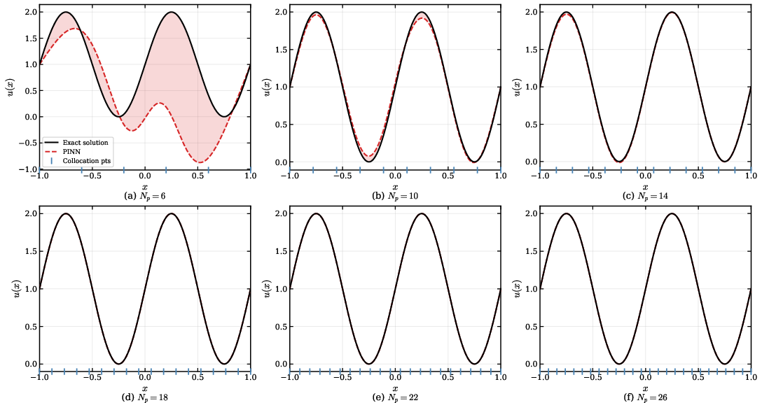
Figure 1: As collocation grid density increases, PINN prediction converges toward the exact solution and $d_{\text{eff}}$4 transitions from saturation (under-resolved) to matching kernel dimension (well-posed).

Subspace Projection: Physics-Preserving Boundary Adaptation

The paper develops a subspace projection strategy for boundary adaptation which updates network parameters strictly within the operator's null space, thereby preserving the learned physics. The protocol is:

1. Physics Null Space Identification: Compute the physics Hessian and its null space via FIM or NTK.
2. Projection: Update boundary-related parameters by projecting them into the operator null space, so modifications cannot degrade the physics constraint.
3. Predictor-Corrector Retraction: Finite precision and manifold curvature induce drift; a corrector step orthogonally projects accumulated error back into the physics null space, preserving residual fidelity.

Empirical results show that subspace projection enables accurate adaptation to new boundary conditions in seconds or minutes, with minimal tuning overhead, achieving competitive BC enforcement and PDE residual compared to gradient-based fine-tuning, which converges more slowly and requires loss balancing and optimizer scheduling.

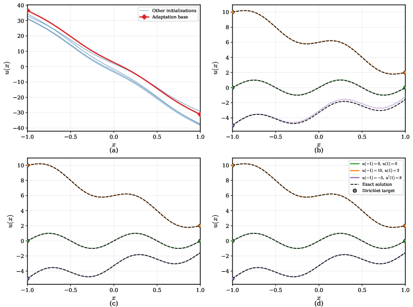
Figure 2: Distinct PINNs trained with varying seeds converge to different physics-satisfying solutions. Subspace projection adapts boundary conditions post hoc without retraining or physics corruption, visualized for both predictor-only and predictor-corrector protocols.

Layer-Wise Adaptation and Multi-Dimensional Extensions

Layer-wise analysis reveals that for 1D problems, the final layer typically anchors the BCs, enabling highly efficient adaptation via least-squares projection. In higher dimensions, e.g., 2D Poisson, the null-space distribution is broader; adaptation scope must scale to additional layers, reflecting representational bandwidth rather than integer invariants. The per-layer $d_{\text{eff}}$5/$d_{\text{eff}}$6 ratio heuristic provides an approximate guide for selecting optimal layers for boundary adaptation.

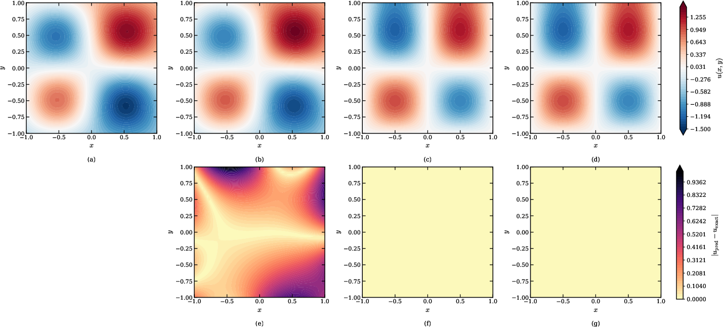
Figure 3: Tanh network adaptation to 2D Poisson: final-layer adaptation yields structured error, penultimate-layer reduces error, adapting both restores accuracy and preserves the solution.

Comparison: Subspace Projection and Fine-Tuning

Subspace projection delivers near-equivalent boundary accuracy to full fine-tuning up to 34$d_{\text{eff}}$7 faster, requiring zero per-problem loss weight tuning. Fine-tuning, while capable of achieving superior asymptotic accuracy, demands prolonged convergence and sensitive hyperparameter scheduling.

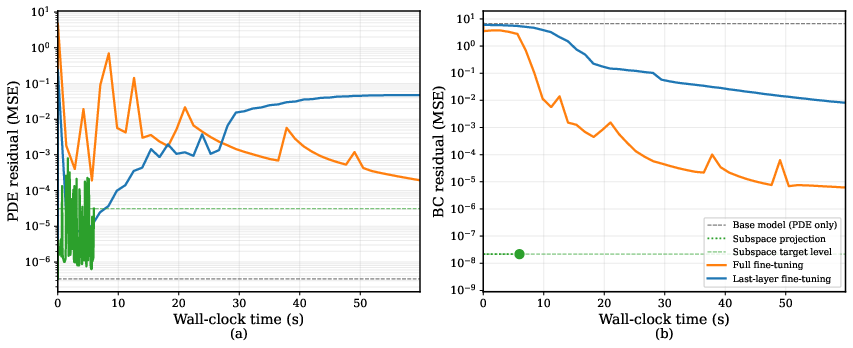
Figure 4: Wall-clock trajectory of PDE MSE and BC MSE for three adaptation strategies; subspace projection achieves rapid BC enforcement while maintaining physics fidelity.

Nonlinear Adaptation: Burgers Equation

In adaptation tasks involving the nonlinear viscous Burgers equation—initial or boundary data shifts triggering shock dynamics—subspace projection accurately reconstructs shock fronts and amplitude changes, outperforming full-grid fine-tuning at comparable compute budgets.

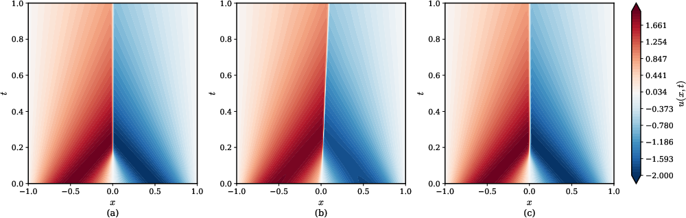
Figure 5: Spatio-temporal contours for initial condition adaptation in Burgers equation. Subspace projection matches shock amplitude and location, while fine-tuning fails to recover amplitude.

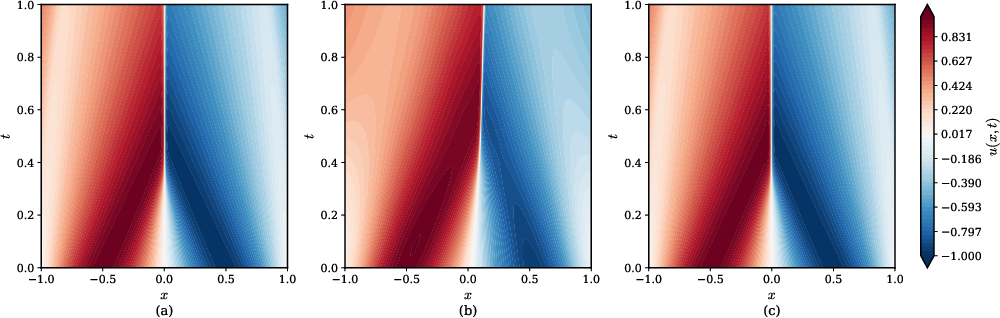
Figure 6: Spatio-temporal contours for time-dependent boundary adaptation in Burgers equation. Subspace projection captures asymmetric shock dynamics; fine-tuning falls short within allotted time.

Implications and Future Directions

Theoretically, $d_{\text{eff}}$8 is recast from a statistical diagnostic to an operator structural invariant, generalizing across architectures and revealing under-resolution independent of loss values. Practically, subspace projection offers a workflow for PINN deployment: pre-train the model on physics, then adapt constraints post hoc in seconds via null-space projection.

Potential future extensions include:

• Low-rank truncation strategies for scaling NTK computations to industrial-scale PDEs.
• Neural architecture search using the null-space structure to eliminate superfluous capacity.
• Uncertainty quantification via sampling in the physics null space.
• Synergistic workflows with operator-learning methods for broad distributional adaptation.

Conclusion

The work rigorously establishes effective dimensionality as an operator invariant and leverages null-space projection for rapid, physics-preserving boundary adaptation in PINNs. Empirical evidence demonstrates architectural invariance, structural diagnostics, and substantial acceleration of boundary adaptation relative to gradient-based methods. The approach lays a foundation for robust, operator-informed scientific machine learning, supporting improved diagnostics, adaptation protocols, and scaling in forward and inverse modeling.