Feature leakage and the identifiability of direct-dependency entropy models of neural activity
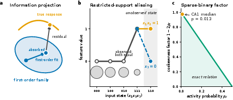
Abstract: Biological neurons receive thousands of synaptic inputs on branching, electrically excitable dendrites, yet population activity is often modeled with direct input-output rules in which each input contributes independently to a scalar drive. We study what successful prediction by such models does, and does not, reveal about neural computation. For conditional maximum-entropy models that match output rates and pairwise output-input coactivities, the entropy explained by a direct model is a prediction measure under the sampled input distribution, not a mechanism-identification test. A restricted MaxEnt fit is an information projection: omitted interaction, temporal, or hidden-state terms can be absorbed into fitted first-order parameters whenever they are correlated with the included sufficient statistics. For sparse correlated binary inputs, this absorption has an explicit coskewness form. We introduce diagnostics that separate in-distribution prediction from recovery of the response rule: state reweighting that holds P(y|x) fixed while changing P(x), conditional log-odds contrasts for local additivity, and temporal leakage controls. In ground-truth simulations, purely higher-order responses can pass first-order entropy and raw coactivity tests under leakage-prone sampling, but are correctly classified after reweighting. Applied to selected, leakage-enriched local tables from CA1 hippocampal recordings, approximately half of tables that appear first-order under empirical weights become distribution-sensitive under balanced reweighting, far above a matched additive-surrogate null. Thus direct entropy-explained fractions and raw coactivity predictions should be interpreted as predictions under the observed state distribution, not as evidence that mechanisms outside the direct model are absent or small.
Paper Prompts
Sign up for free to create and run prompts on this paper using GPT-5.
Top Community Prompts
Explain it Like I'm 14
What this paper is about (in simple terms)
Imagine a neuron as a light bulb that turns on or off depending on many on/off switches (its inputs). A common, simple idea is that each switch adds its own little push, and the bulb turns on if the total push is big enough. But in real brains, switches can team up: two switches together might have an effect that neither has alone.
This paper asks: if a simple “add up the switches” model seems to predict a neuron’s activity well, does that mean the neuron truly works that way? Their main message: good prediction by a simple model does not necessarily mean the neuron is truly simple. Hidden teamwork among inputs can “leak” into the simple model and make it look better than it should.
The key questions, made easy
- Can a simple model that adds up inputs really explain a neuron’s behavior?
- If it can, does that prove the neuron has no special team-up (interaction) effects?
- How can we tell the difference between “the neuron is truly simple” and “the data made a complex neuron look simple”?
How they studied it (everyday explanation)
They focus on a kind of model called a “conditional maximum-entropy” model. You can think of it as:
- We match a few easy-to-measure facts (like how often the neuron fires and how often it fires when each input is on).
- Then we choose the simplest possible rule that fits those facts.
- That rule ends up looking like “add up each input’s weight and pass it through a squashing function,” which is basically a classic additive model.
Why might this be misleading? Two big reasons:
- Feature leakage (inputs teaming up can masquerade as single-input effects):
- Picture two switches that often turn on together. If you ignore their teamwork but they happen to be synced in your data, a model that only looks at single switches can still look great—because each switch is acting as a stand-in for their team effect.
- This is especially strong when inputs are on/off (binary) and rarely on (sparse), like most neurons that are silent most of the time. In such data, teamwork effects can “project” onto single inputs very easily, making a simple model seem smart even if it ignores the teamwork.
- Skewed sampling (seeing only certain combinations of switches):
- If your recording happens to see some input combinations a lot and others almost never, your model may look good on what you saw, but fall apart if the input combinations change.
To separate “true simplicity” from “looks simple because of the data,” they designed three practical checks:
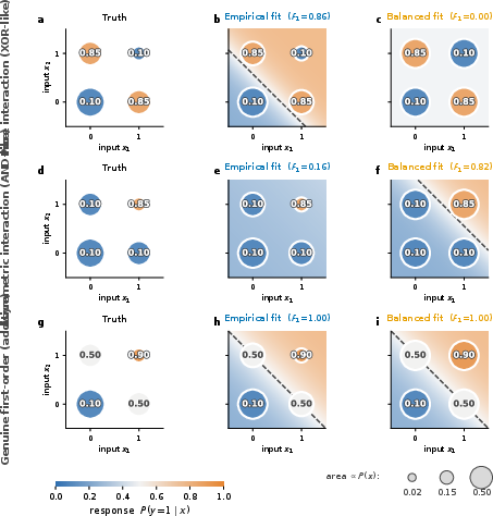
- Change the input mix without changing the response (state reweighting): Keep the neuron’s response table fixed (how likely it is to fire for each on/off combination of a few inputs), but pretend the world shows all combinations more evenly. If the simple model still does well, the neuron is likely truly simple. If the model now struggles, it was riding on the original data’s quirks.
- Check additivity directly with a simple contrast: They compute a number from the response table that is zero if effects just add up, and nonzero if there’s teamwork (interaction). This targets the actual response rule, not the frequency of states.
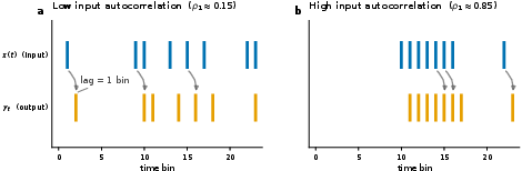
- Test for time leakage: If present-time inputs are similar to recent past inputs, then a model that only uses “now” can seem to predict delayed effects. They simulate this to show how an instantaneous model can look good even when the true rule is delayed.
They tried all of this first in simulations where they know the true rule, and then on real brain data from mouse hippocampus (CA1) and visual cortex.
What they found and why it matters
Main findings from simulations:
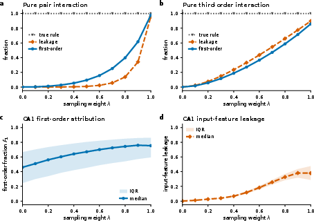
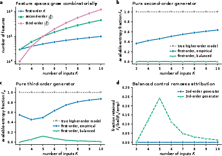
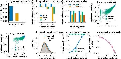
- The same complex neuron (with real teamwork between inputs) can look simple if inputs are sparse, binary, and correlated. In those conditions, the simple model can capture a large fraction of the “explainable” behavior—even though it’s structurally wrong.
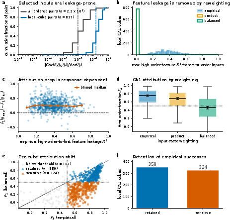
- When they reweight the input states to be more balanced (pretend all combinations are seen equally), the simple model’s success often drops sharply for these complex neurons. That shows the earlier success was partly an illusion caused by the sampling.
- A direct additivity test on the response table catches genuine teamwork even when the simple model’s predictions looked good under the original sampling.
- For time-delayed effects, strong input autocorrelation lets a model with only “now” inputs predict delayed co-activity—again, a misleading success.
Findings on real data (local, well-sampled subsets):
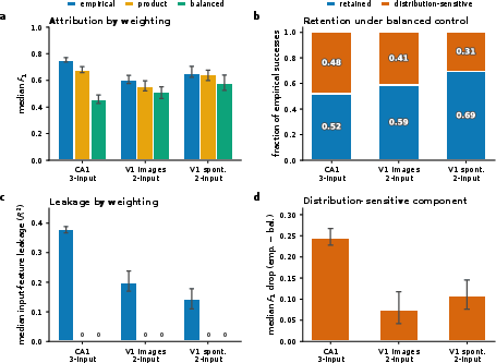
- Hippocampus (CA1): They examined many small “local tables” (a neuron’s response to 2–3 of its inputs, all on/off combinations). Under the original data’s input mix, a simple additive model often looked very good. But when they reweighted the inputs to be balanced, about half of the cases that looked simple no longer did. This means the simple model’s success depended on the particular input patterns that were most common in the recording.
- Importantly, this is not due to random noise: when they built fake data from truly additive neurons, the reweighting did not cause the same drop.
- Visual cortex showed a smaller version of the same effect, suggesting the issue is general but varies by dataset.
Why this matters:
- Many studies judge models by how well they predict averages like “how often do three cells fire together.” The paper shows such tests are descriptive, not decisive for mechanism. A simple model can match those averages because of the input mix, not because the neuron truly adds inputs independently.
- So, “high entropy explained” or “co-activities predicted” is about being good under the observed conditions—not proof that more complex neuron mechanisms are absent.
What this means going forward
- Don’t equate good prediction by a simple model with proof that the brain itself is simple. The data’s patterns can hide teamwork between inputs.
- Use diagnostic checks:
- Reweight input states to see if the model’s success is stable.
- Use simple additivity contrasts on the response table to detect teamwork directly.
- Check for time-leakage when inputs are autocorrelated.
- Practical takeaway: Direct, additive models are useful for prediction under the conditions you measured. But they are not reliable “mechanism detectors” unless you also show their success doesn’t vanish when the input distribution changes, and unless they pass direct additivity tests.
Short summary
- Problem: Simple “add the inputs” models often look great at predicting neuron activity.
- Hidden issue: In sparse, on/off neural data, input teamwork can masquerade as single-input effects, and uneven sampling can boost this illusion.
- Solution: Test stability by reweighting input states, measure additivity directly, and watch for time leakage.
- Result: In real hippocampal data, about half of seemingly simple cases lost their “simplicity” under balanced reweighting; similar but smaller effects appeared in visual cortex.
- Bottom line: Great prediction does not equal true mechanism. Interpret “explained entropy” and co-activity fits as “works under these data conditions,” not as proof that interactions are absent.
Knowledge Gaps
Knowledge gaps, limitations, and open questions
Below is a concise list of unresolved issues that future work could address to strengthen identifiability claims and broaden the applicability of the framework.
- Scope beyond small local tables: the diagnostics are demonstrated on 2–3 input “cubes”; it remains unclear how to scale reweighting and conditional-odds tests to realistic high-dimensional input sets without prohibitive sample-size demands.
- Finite-sample reliability under reweighting: no systematic analysis of estimator variance, bias, and confidence intervals for reweighted entropy fractions; practical sample-size requirements and variance-control strategies (e.g., shrinkage, Bayesian smoothing) are not quantified.
- Support mismatch in high dimensions: the method requires overlap between empirical and target weights; strategies for safe reweighting when balanced/product weights place mass on rarely or never observed states are not developed.
- General-purpose importance weighting: no algorithmic framework for learning a family of plausible P(x) reweightings (beyond product and fully balanced) that maximize power to expose leakage while controlling variance.
- Identification bounds: while absorbed effects cannot be bounded without curvature lower bounds (Schur complement), the paper does not propose practical ways to estimate or lower-bound I_GG|F from data, leaving only qualitative identifiability statements.
- Estimating leakage magnitude: there is no dataset-level estimator for the absorbed component of omitted structure (e.g., via proxies for G or sensitivity analyses) to quantify how much of the “first-order” fit is due to leakage.
- Diagnostic power vs. smoothing choices: the effect of different smoothing/regularization schemes on Δ_ij and F1 decisions is not characterized; guidelines for robust hyperparameter selection are missing.
- Multiple testing and selection bias: cubes are selected for leakage-prone geometry; there is no correction for multiple comparisons or a plan to obtain unbiased prevalence estimates across all triplets/neuron subsets.
- Generalization beyond binary outputs: the framework assumes a binary output; extensions to graded firing rates or count models (e.g., Poisson/negative-binomial GLMs) are not analyzed.
- Sensitivity to binarization thresholds: binarization collapses single-input nonlinearities; the impact of threshold choice, bin width, and spike-inference errors on leakage and identifiability is not quantified.
- Alternatives to binarization: whether using continuous features, multi-level discretization, or orthogonalized bases reduces coskewness leakage is not tested.
- Temporal structure in real data: the temporal-leakage control is shown in simulation only; there is no quantification of instantaneous-vs-lagged absorption in CA1 or V1 recordings.
- History effects and refractory dynamics: the framework focuses on instantaneous features; extensions to rich history-dependent GLMs and their identifiability under autocorrelation are not explored on real data.
- Hidden-state confounds: the role of unobserved modulatory variables (arousal, behavioral state) in creating apparent first-order attribution via correlations with F is acknowledged but not modeled; no latent-variable or deconfounding strategy is provided.
- Causal/experimental tests: there is no intervention-based validation (e.g., optogenetic decorrelation, controlled stimulation) to change P(x) and test whether first-order attribution remains stable across contexts.
- Design-of-experiments: no guidance on how to design perturbations that optimally break Fisher cross-covariances I_FG and maximize identifiability of interactions under practical constraints.
- Theoretical conditions for orthogonality: concrete, testable sufficient conditions on P(x) under which Fisher-orthogonality (I_FG=0) holds for realistic neural statistics are not derived.
- Measuring coskewness leakage in practice: while a binary coskewness identity is given, the paper does not provide a robust estimator or diagnostic for “leakage propensity” at scale (e.g., per-neuron or per-pair indices with uncertainty).
- Relationship to raw coactivity pipelines: the work shows raw coactivities are descriptive, but does not propose a corrected coactivity metric that targets conditional mechanisms while remaining computationally tractable.
- From local to global models: it remains open how local non-additivity and distribution sensitivity aggregate within full neuron-level models (greedy dictionaries, GLMs) and whether local diagnostics predict global transfer failures.
- Cross-dataset breadth: only CA1 (3-input) and V1 (2-input) datasets are analyzed; broader tests across brain areas, tasks, species, and recording modalities are needed to assess generality.
- Structural correlates: there is no analysis linking distribution-sensitive tables to anatomical, spatial, or cell-type features (e.g., dendritic location, inhibitory/excitatory identity) that could ground mechanistic hypotheses.
- Model class limitations: only additive-logistic (conditional MaxEnt) families are studied; comparisons to alternative direct models (e.g., probit, spline-based, or spike-and-slab GLMs) and their identifiability properties are missing.
- Quantifying practical impact: the downstream consequences of leakage for common inferences (functional connectivity, feature selection, decoding) are not evaluated.
- Reweighting under nonstationarity: how to perform state reweighting when P(x) changes over time (behavioral epochs, drift) without conflating context shifts with identifiability is not addressed.
- Autocorrelation dependence: precise characterization of how much temporal autocorrelation suffices for instantaneous statistics to explain delayed coactivities (with confidence bounds) is not provided.
- Interaction order and dimensionality: simulations show leakage grows with input count K for fixed-order generators; empirical tests at higher orders (>3 inputs) in real data are absent due to sampling limits—methods to overcome this are needed.
- Quantitative thresholds: choices for classifying “retained” vs. “distribution-sensitive” are somewhat arbitrary; principled, power-calibrated thresholds or decision criteria are not formalized.
- Inference of G from data: strategies to discover which interaction or lag features (G) are most responsible for leakage (e.g., via targeted residual modeling or conditional tests) are not developed.
- Robustness to preprocessing: the impact of deconvolution quality, motion correction, and neuropil contamination (in calcium data) on the leakage diagnostics is not measured.
- Practical tooling: while an analysis package is mentioned, there is no formal benchmarking suite or standardized workflow for practitioners to diagnose leakage and report uncertainty in new datasets.
Practical Applications
Immediate Applications
The following applications can be deployed now by incorporating the paper’s diagnostics, cautions, and workflows into existing analysis and modeling pipelines.
- Academia (neuroscience data analysis)
- Add identifiability diagnostics to MaxEnt/GLM studies on neural data
- Workflow: alongside fitting direct (first-order) conditional MaxEnt/GLM models, run (a) state reweighting (empirical → product-marginal → balanced), (b) conditional log-odds contrasts (Δ_ij) to test additivity, (c) temporal leakage checks (lagged vs instantaneous features), and (d) additive-surrogate nulls to calibrate finite-sample baselines.
- Tools/products: “Reweight-and-refit” module; “Conditional odds-contrast” function; “Temporal leakage stress test” for time series; “Additive-surrogate null” simulator; “Feature-leakage score” based on coskewness projection.
- Dependencies/assumptions: adequate sampling of local input states (e.g., 2–3 inputs) to support exact reweighting; stability of P(y|x) across reweightings; variance control and smoothing for rare states; careful cross-validation.
- Report predictive vs mechanistic claims separately
- Workflow: explicitly label entropy-explained and raw coactivity metrics as prediction under P(x); move mechanism claims to P(x)-invariant diagnostics (Δ_ij) and cross-distribution tests.
- Dependencies/assumptions: discipline-wide adoption of reporting standards; willingness to include additional control analyses.
- Software/ML engineering (binary/sparse-feature modeling)
- Distribution-sensitive model validation for logistic/MaxEnt/GLMs on sparse binary data
- Use case: recommender systems, fraud detection, ad-click models, medical risk scoring with many binary indicators.
- Workflow: add reweighting (to product-marginal/balanced) and “leakage” projections to CI tests; test stability of first-order attribution, and when unstable, introduce interaction or lag features; quantify dataset shift risk.
- Tools/products: scikit-learn/PyTorch add-ons for reweighting, coskewness-based leakage scoring, Δ_ij-like contrasts in generalized settings; model cards noting distribution sensitivity.
- Dependencies/assumptions: ability to approximate or synthesize alternative P(x); sufficient data to avoid high-variance reweighting; governance for evaluating models under counterfactual state weights.
- Temporal leakage guardrails in time-series modeling
- Use case: demand forecasting, user-behavior prediction, medical monitoring where autocorrelation can let instantaneous models mimic lagged effects.
- Workflow: run lag-aware vs instantaneous feature comparisons; evaluate held-out likelihood gains and delayed coactivity prediction across autocorrelation sweeps; flag when instantaneous features likely absorb lag mechanisms.
- Dependencies/assumptions: lag feature engineering; stationarity over evaluation windows; robust cross-validation across lags.
- Experimental neuroscience and lab workflows
- Balanced/perturbative stimulus design to probe identifiability
- Use case: imaging/ephys experiments in which inputs can be partially controlled (visual stimuli, optogenetic perturbations).
- Workflow: introduce stimuli or perturbations that decorrelate inputs (approximate product-marginal or balanced P(x)); sample “rare corners” of the input cube; repeat direct-model fits under multiple P(x) to see whether first-order attribution is stable.
- Dependencies/assumptions: feasibility of controlled perturbations; ethical/technical limits; sufficient trials to populate rare states.
- Brain–computer interfaces (healthcare/neurotech)
- Robust decoder validation across state distributions
- Workflow: validate BCI decoders by reweighting or re-collecting sessions under different behavioral/cognitive states; check whether direct linear decoders retain performance or require interaction/lag terms.
- Tools/products: “state-weight stress test” in BCI calibration suites; Δ_ij-like checks to detect non-additivity in neural features.
- Dependencies/assumptions: access to multiple behavioral contexts; stability of decoder training; monitoring of nonstationarity.
- Finance and marketing analytics
- Causally cautious interpretation of GLM coefficients on click/risk events
- Workflow: apply reweighting and leakage diagnostics to distinguish predictive success from mechanistic inference; prioritize experimentation (A/B tests) or targeted decorrelation when mechanism matters.
- Dependencies/assumptions: logging of sufficient covariates; ability to run controlled experiments; careful handling of rare-event variance.
- Policy, epidemiology, and social science
- Guard against overinterpreting additive models on observational, sparse data
- Workflow: report that “direct” (first-order) model fit is predictive under observed P(x); perform P(x)-invariant interaction tests and reweighting sensitivity analyses before making mechanism claims; prefer interventions when possible.
- Dependencies/assumptions: high-quality observational data; estimable alternative P(x); institutional appetite for conservative claims.
- Publishing and peer review standards
- Checklists for identifiability claims in MaxEnt/GLM papers
- Workflow: require authors to run and report state reweighting, Δ_ij contrasts, temporal leakage controls, and additive-surrogate nulls when asserting additivity or absence of higher-order mechanisms.
- Dependencies/assumptions: community consensus and journal adoption.
- Education and training
- Incorporate “prediction vs mechanism” modules into methods curricula
- Workflow: lab exercises implementing reweighting, Δ_ij, and temporal leakage on open datasets; emphasize information projection and Schur-complement residuals.
- Dependencies/assumptions: accessible teaching code and datasets.
Long-Term Applications
These applications require further research, development, scaling, or new data acquisition capabilities.
- Identifiability-aware analysis platforms (software)
- Product: integrated libraries that estimate Fisher cross-blocks (I_FF, I_FG), Schur-complement residuals, and leakage bounds; automatically generate state-weight tuning curves and “leakage dashboards”; recommend minimal interaction/lag features to recover residuals.
- Dependencies/assumptions: efficient and stable estimation in high dimensions; approximate inference for large models; user interfaces for non-experts.
- Closed-loop experimental design to actively disambiguate mechanisms
- Product: controllers that adapt stimuli/perturbations to sample input states that maximally separate additive vs interaction models (e.g., target rare corners).
- Dependencies/assumptions: real-time inference; safe perturbation bandwidth (e.g., optogenetics); hardware latency and ethical constraints; robust stopping criteria.
- Large-scale neural recording protocols that minimize leakage-prone regimes
- Innovation: recording methods and preprocessing that avoid aggressive binarization (retain graded activity), improve coverage of input state space, and explicitly log external/contextual variables to reduce hidden-state absorption.
- Dependencies/assumptions: advances in sensor density, stability, and analysis pipelines; storage/compute scale; standardized metadata.
- Model selection and AutoML that accounts for feature leakage
- Product: AutoML systems that diagnose when first-order models will absorb interactions under observed P(x), suggest targeted interaction/lag terms, and propose data augmentation or sampling strategies to reduce leakage.
- Dependencies/assumptions: reliable proxies for leakage in non-binary, high-dimensional feature spaces; safe reweighting or augmentation at scale; integration with production ML workflows.
- Robust BCI and clinical decision systems with identifiability monitors
- Product: decoders with built-in alarms for distribution-sensitive attribution; automatic recalibration to maintain mechanism-robust performance across contexts; logging for regulatory audits distinguishing predictive vs mechanistic claims.
- Dependencies/assumptions: regulatory pathways; clinical validation; patient safety frameworks; long-term stability across sessions.
- Safety assessments for robotics and offline RL via reweighting diagnostics
- Use case: value/policy models trained off-policy may “explain” data under logged P(x) while misrepresenting mechanisms.
- Workflow/product: evaluation harness that reweights or simulates alternate state-action distributions to test stability of learned dependencies; flags interactions/temporal terms needed for safe deployment.
- Dependencies/assumptions: accurate estimators for alternative state-action visitation; simulators or logged data breadth; robust off-policy evaluation.
- Cross-domain standardization and benchmarks
- Product: public benchmark suites with datasets spanning multiple P(x) contexts (empirical, product-marginal, balanced), plus gold-standard interaction/lag ground truths; leaderboards for identifiability-aware metrics (beyond raw coactivity R2).
- Dependencies/assumptions: community coordination; dataset curation; sustainable hosting and governance.
- Policy frameworks for mechanism claims from observational models
- Product: guidance and standards (e.g., in epidemiology/economics) requiring distribution-sensitivity analyses before mechanism-based policy recommendations; templates to communicate prediction vs mechanism to stakeholders.
- Dependencies/assumptions: institutional buy-in; training for practitioners and reviewers; alignment with causal inference best practices.
- Targeted data collection in high-stakes analytics (finance, cybersecurity, health)
- Workflow: active data acquisition to decorrelate key binary indicators (e.g., synthetic probes, controlled tests) to reduce coskewness-driven leakage; incorporate lag-disambiguation experiments.
- Dependencies/assumptions: operational feasibility of interventions; risk management; compliance constraints.
Each long-term direction leverages the paper’s core insights: (1) direct-model success under a given P(x) is a statement about prediction, not mechanism; (2) omitted features can be absorbed through information projection (I-projection) when correlated with included statistics; and (3) reweighting, conditional odds-contrasts, and temporal leakage tests provide practical paths to mechanism-aware conclusions.
Glossary
- Additive logistic unit: A model component where inputs contribute linearly to log-odds and a logistic nonlinearity maps to output probability. Example: "It cannot distinguish, on its own, whether biological neurons nonlinearly integrate synaptic information or are effectively additive logistic units under the sampled conditions."
- Additive-surrogate null: A simulated additive model used as a baseline to test whether observed effects could arise from estimation noise. Example: "an effect far above a matched additive-surrogate null."
- Autocorrelation: The correlation of a signal with a time-shifted version of itself, here used to relate present and past neural activity. Example: "As lag-one autocorrelation increases, the instantaneous model increasingly passes the lagged-coactivity metric, reaching at autocorrelation $0.98$, even though the ground truth is purely lagged."
- Balanced reweighting: A control that evaluates models under a uniform distribution over input states to test distribution sensitivity. Example: "approximately half of those that appear first-order under empirical weights become distribution-sensitive under balanced reweighting, an effect far above a matched additive-surrogate null."
- Balanced sampling: Using equal weights for all input states when evaluating a response table. Example: "but not under balanced sampling ()."
- Bernoulli entropy: The entropy of a Bernoulli random variable, used to compute model entropy. Example: "where is the Bernoulli entropy."
- Binarization: Converting continuous activity to binary (0/1) variables, which can collapse nonlinearities. Example: "Binarization collapses positive powers of a single input because on for all ."
- CA1 (hippocampal area CA1): A subregion of the hippocampus from which neural recordings were analyzed. Example: "We apply the diagnostics to selected, leakage-enriched local tables from CA1 hippocampal recordings."
- Conditional entropy: The expected uncertainty of an output given inputs; used to assess model prediction. Example: "the conditional entropy of the fitted direct model"
- Conditional log-odds contrasts: Tests based on differences in log-odds across input conditions to assess additivity. Example: "(2) conditional log-odds contrasts that test additivity of the local response table;"
- Conditional maximum-entropy (MaxEnt): Modeling approach that chooses the least-structured conditional distribution consistent with specified moments. Example: "We study this question for conditional maximum-entropy (MaxEnt) models that match the output rate and pairwise output-input coactivities."
- Coskewness: A third-order moment measuring how two variables’ product covaries with a third; here, how interaction features project onto first-order terms. Example: "For sparse correlated binary inputs, this absorption has a simple coskewness form that we derive explicitly."
- Dendritic nonlinearities: Nonlinear integration phenomena occurring in dendrites (e.g., due to active conductances). Example: "Related cautions about restricted maximum-entropy population models, coupled GLMs, higher-order correlations, dendritic nonlinearities, and activity-based connectivity inference appear in prior work"
- Direct-dependency conditional MaxEnt model: A MaxEnt model that assumes additive dependence of output on selected inputs (no explicit interactions). Example: "Here, we develop an identifiability framework for direct-dependency conditional MaxEnt models of neural activity."
- Exponential family: A class of probability distributions characterized by sufficient statistics and natural parameters; MaxEnt models are members. Example: "The identifiability argument below uses standard information-geometric notions of -projection onto an exponential family"
- Fisher information (conditional Fisher covariance blocks): Expected curvature (covariance of score functions) quantifying parameter sensitivity; blocks defined over included/omitted statistics. Example: "Define the conditional Fisher covariance blocks at :"
- Fisher-orthogonality: A condition where included and omitted sufficient statistics have zero Fisher cross-covariance, preventing leakage. Example: "No leakage requires Fisher-orthogonality between the included and omitted sufficient statistics under the sampled input distribution."
- Greedy-dictionary analysis: A forward-selection procedure over a dictionary of features to assess model improvements. Example: "A complementary greedy-dictionary analysis and a larger check gave the same qualitative result"
- Held-out negative log-likelihood (NLL): A predictive performance metric computed on data not used for fitting. Example: "and the held-out negative log-likelihood (NLL) gap between direct and interaction models remains positive"
- I-projection: The information projection of a distribution onto a constrained family by minimizing KL divergence. Example: "The identifiability argument below uses standard information-geometric notions of -projection onto an exponential family"
- Identifiability: The ability to uniquely infer model structure/mechanism from data; central to distinguishing prediction from mechanism. Example: "Here, we develop an identifiability framework for direct-dependency conditional MaxEnt models of neural activity."
- Information geometry: The differential-geometric study of statistical models using concepts like I-projection and Fisher information. Example: "The identifiability argument below uses standard information-geometric notions of -projection onto an exponential family"
- Information projection: Fitting a restricted MaxEnt model by projecting the true distribution onto the model family under the observed input distribution. Example: "A restricted MaxEnt fit is an information projection under the sampled input distribution."
- Lagrange multipliers: Parameters enforcing constraints (e.g., moments) in MaxEnt models; here, the fitted weights. Example: "fitted direct parameters are Lagrange multipliers for activity statistics, not causal synaptic parameters."
- Latent model: A generative model with hidden variables used here to induce input correlations. Example: "Inputs are generated from a one-factor latent model with tunable correlation "
- Logit: The logarithm of odds; linear in inputs for additive logistic models. Example: "logit P(y=1\mid x)=Kx_1x_2"
- Odds-ratio contrast: A statistic comparing log-odds across input conditions to detect interactions. Example: "The more direct local test is a conditional odds-ratio contrast."
- Product-marginal control: A reweighting that uses the product of input marginals to remove dependencies while preserving individual rates. Example: "(using a mild product-marginal control and a balanced stress-test endpoint)"
- Rare-corner sampling: An input-state distribution where certain joint states (e.g., “11”) are extremely infrequent, potentially masking interactions. Example: "A pure XOR-like interaction is well described by a first-order readout under empirical rare-corner sampling ()"
- Schur complement: A matrix operation describing residual information after projecting out included statistics. Example: "The residual detectable by the restricted family is governed by the Schur complement"
- State reweighting: Changing the weights of input states while holding the response table fixed to test distribution sensitivity. Example: "a state-reweighting control that holds fixed while changing "
- Sufficient statistics: Functions of data that capture all information about parameters within an exponential-family model. Example: "These models provide a principled measure of prediction by first-order sufficient statistics."
- Temporal leakage: Absorption of lagged (time-delayed) mechanisms by instantaneous statistics due to temporal correlations. Example: "and (3) a temporal leakage simulation that quantifies when instantaneous statistics absorb lagged mechanisms."
- Time-delayed coactivities: Joint activity patterns involving delayed inputs and current outputs. Example: "raw higher-order and time-delayed coactivities"
- XOR-like interaction: A non-additive interaction where output depends on the parity (exclusive OR) of inputs. Example: "A pure XOR-like interaction is well described by a first-order readout under empirical rare-corner sampling ()"
Collections
Sign up for free to add this paper to one or more collections.