Universal Time Series Generation with Neural Controlled Differential Equations
Abstract: Recent work on the sequence universality of State Space Models (SSMs) has introduced efficient, maximally expressive continuous-time approaches for time-series modelling. While these works focus on discriminative settings, we extend this perspective to generative time-series modelling by proving that maximally expressive Structured Linear Controlled Differential Equations (SLiCEs) are universal time-series generators, in the sense that they can approximate the induced path laws of continuous causal pushforwards on compact latent sets in $W_\infty$. Building on these theoretical results, we propose Generative SLiCEs (G-SLiCEs), a maximally expressive continuous-time model for flow matching on path-space. Empirically, we show that expressivity improves performance in probabilistic forecasting and downstream tasks, while retaining the advantages of continuous-time models such as generalising to arbitrary observation grids. This is particularly beneficial for irregular grids, where fixed-grid models often struggle.
Paper Prompts
Sign up for free to create and run prompts on this paper using GPT-5.
Top Community Prompts
Explain it Like I'm 14
What is this paper about?
This paper is about teaching computers to generate realistic time series — sequences that change over time, like temperature every hour, electricity demand every minute, or traffic speed every second. The authors introduce a new model, called G-SLiCE, that works in continuous time (not just at fixed steps) and prove that it is “universal,” meaning it can learn to produce almost any kind of time series pattern if given enough capacity and the right training. They also show it works well in practice, especially when data are recorded at uneven times.
What were the researchers trying to do?
Here are the main goals, written simply:
- Build a time-series generator that is both expressive (can learn many kinds of patterns) and efficient (fast and stable to run).
- Prove a strong guarantee: if the model can imitate any path-by-path rule, then it can also imitate any distribution of paths (any “style” of time series) — this is called universality for generation.
- Turn that theory into a practical method that learns flows on entire paths, not just on single time points.
- Show in experiments that the new method beats strong baselines on probabilistic forecasting and stays accurate even when the observation grid (the sampling times) changes.
How did they do it? (Methods in simple terms)
The authors combine three big ideas. Here they are with everyday analogies:
Time series as paths in continuous time
- Instead of only looking at values at fixed steps (like every hour), the model treats a time series as a continuous path — a smooth curve over time. This helps when measurements arrive at weird, uneven times.
SLiCE: a structured “state tracker”
- Think of the model as a machine with an internal “state” (like a memory) that gets updated as time moves forward. This update is guided by a set of simple rules that are linear in the state but read the input path continuously. This kind of model is called a Neural Controlled Differential Equation (NCDE).
- “Structured Linear CDEs” (SLiCEs) add structure to the internal matrices (like making them block-diagonal or diagonal-plus-low-rank). This keeps them fast and stable without losing expressiveness.
- Even though the state updates are linear, the overall behavior can be very rich because the model is driven by the changing input path.
Flow matching on path space: morphing noise into data
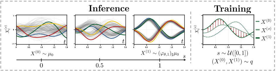
- To generate new time series, the model starts from a “noise path” and learns a smooth way to turn it into a realistic path. Imagine morphing a rough sketch into a finished drawing, not just moving a single dot but the whole curve over time.
- The starting noise path comes from a Gaussian process (a standard way to draw random, smooth curves).
- The model learns a “vector field” — a rule that says how to nudge the entire path at each step of a fictitious flow time s from 0 to 1 so that, by the end, the path looks like real data.
- During training, the model sees pairs of noise paths and real paths and is asked: “If I interpolate between these two, what direction should I push the current path to reach the real one?” That training style is called conditional flow matching.
A few helpful terms:
- Causal: the model only uses the past to predict the present (no peeking into the future).
- Pushforward: take randomness from a simple source (the noise paths) and pass it through the model to get randomness in the form you want (realistic time series).
- Universality (here): the model class can approximate any reasonable time-series distribution as closely as we like.
What did they find?
The authors present both theoretical guarantees and practical results.
- Theory: They prove that if a model can approximate any path-to-path rule (causal and continuous), then it can also approximate any distribution over paths (the “styles” of time series). Using this, they show that maximally expressive SLiCEs are universal generators on path space. In short: great at imitating rules implies great at imitating distributions.
- New model (G-SLiCE): They build a generative model that uses SLiCE as its backbone and trains via flow matching to morph noise paths into data-like paths.
- Experiments:
- Probabilistic forecasting: G-SLiCE achieves state-of-the-art or improved performance compared to strong baselines, including recent flow- and diffusion-based methods.
- Robust to grid shifts: Because it works in continuous time, G-SLiCE handles irregular or shifted sampling times better than fixed-grid models.
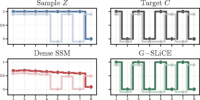
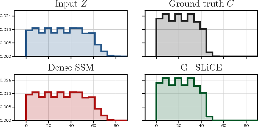
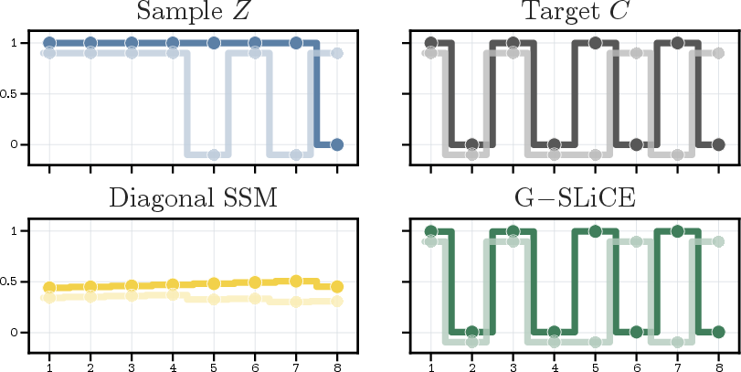
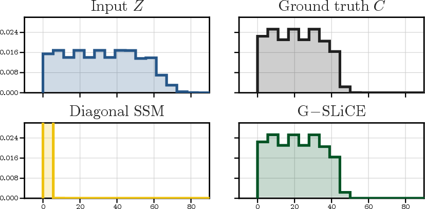
- Expressivity gap example: They show a simple task where some popular, efficient models with too-restricted internal structure (like only diagonal transitions or time-only updates) cannot capture certain “state-tracking” patterns. G-SLiCE can, highlighting why expressivity matters.
Why this is important:
- Better expressivity means the model can learn subtle, state-dependent rules (e.g., “don’t place two 1s in a row”), which some simpler models miss.
- Continuous-time modeling means the same model works whether your data are evenly spaced or irregular — no special handling needed.
Why does this matter?
- Practical impact: In areas like weather forecasting, energy demand, and traffic, it’s crucial not just to predict one future value, but to model the full range of possible futures (probabilistic forecasting). G-SLiCE is designed exactly for that and performs well.
- Handles messy real-world data: Many real datasets have missing or irregular sampling. Continuous-time models like G-SLiCE naturally deal with this.
- Strong foundation: The universality guarantees suggest that if you scale the model and train it well, it can learn the kinds of distributions practitioners care about — not just isolated points.
- Efficient and parallel: Its structured design keeps it computationally attractive, allowing parallel-in-time computation while remaining expressive.
In short, this paper builds a bridge between powerful theory and practical, robust tools for generating realistic time series. The result is a model that not only works well in experiments but also comes with convincing reasons why it should work across many situations.
Knowledge Gaps
Knowledge gaps, limitations, and open questions
Below is a single, consolidated list of what remains missing, uncertain, or unexplored in the paper, formulated to be concrete and actionable for future research.
- Universality under non-compact and heavy-tailed latent laws: The main generative universality result requires compactly supported latent path laws; the paper sketches high-probability statements for Gaussian-process priors but does not provide formal guarantees or rates for non-compact, heavy-tailed, or non-Gaussian priors.
- Continuity requirement of target maps: Universality is proven only for continuous causal pushforwards; many practical mappings (e.g., thresholding, regime switches, interventions) are discontinuous. Extending path-space universality to measurable, discontinuous causal maps remains open.
- Integration and path regularity assumptions: All results assume absolutely continuous inputs and Riemann–Stieltjes integration. Real-world time series often exhibit jumps, impulsive events, or rough paths. A rough-path or Skorokhod-space generalization with corresponding universality guarantees is missing.
- Discretization error and its effect on universality: The theory is continuous-time, but training and inference operate on discretized grids. Quantifying how discretization (including interpolation and augmentation) degrades guarantees and characterizing error-vs-step-size trade-offs is not addressed.
- Training guarantees for path-space flow matching: The flow-matching objective (with straight-line interpolants and mini-batched optimal transport coupling) lacks convergence guarantees, sample complexity bounds, or conditions ensuring consistency in path-space. A theoretical analysis of optimization and generalization for the proposed training scheme is absent.
- Impact of coupling choice in path-space: Mini-batched optimal transport is adopted without analyzing its bias, variance, or stability on infinite-dimensional path-space; the sensitivity to batch size, coupling suboptimality, and computational scaling is not studied.
- Prior mismatch and kernel selection: Using Gaussian-process priors (and conditional GPs) is justified heuristically, but the paper does not study how kernel choice, hyperparameter misspecification, or prior–data mismatch affect generative performance or theoretical guarantees.
- Stability and well-posedness of the path-space flow: Conditions ensuring existence, uniqueness, and stability of the learned ODE in flow time (e.g., Lipschitz bounds on the SLiCE vector field, matrix-exponential stability, gradient stability during training) are not provided.
- Efficiency vs. expressivity trade-offs: While SLiCE structures are touted as both expressive and efficient, there is no quantitative complexity analysis (time/memory) comparing block-diagonal, diagonal-plus-low-rank, sparse, or Walsh–Hadamard variants against S4/Mamba across sequence length, channel dimension, and grid irregularity.
- Robustness to grid shifts and irregular sampling: Empirical claims of robustness are not backed by formal invariance analysis (e.g., under time warping, resampling, missingness patterns). A systematic stress test and theoretical characterization of robustness to arbitrary grid perturbations are lacking.
- Extent of expressivity separations: The negative results target single-layer diagonal or non-selective transitions. It remains open whether stacking, nonlinear projections, or hybrid structures (e.g., selective diagonal-plus-low-rank) recover continuous causal path-to-path universality (not just discrete sequence-to-sequence).
- Augmentation design and causality: The proofs assume deterministic causal augmentations (time, masks, lags), but there is no formal guidance on augmentation design, nor analysis of how specific choices impact universality, stability, or causality preservation.
- Metric choice beyond : The theory uses on the supremum metric; practical forecasting often evaluates CRPS, (for ), or weak convergence. Extending universality and approximation guarantees to other metrics relevant for forecasting is needed.
- Constraints and non-Euclidean paths: Many time series live on constrained manifolds (positivity, periodicity, conservation). While manifold flow matching is cited, G-SLiCE does not incorporate constraints or provide universality on manifold-valued path-spaces.
- High-dimensional, multivariate dependencies: The paper does not analyze cross-channel causality, contemporaneous dependence, or conditional generation with exogenous covariates (beyond deterministic augmentation), leaving open whether universality and training scale with dimension and complex dependencies.
- Likelihoods and tractable densities: The deterministic path-space flow suggests potential for continuous normalizing flow-style likelihoods on path-space, but the paper does not address whether densities or log-likelihoods are tractable, nor how to perform likelihood-based training.
- Handling observation noise and partial observability: Conditional generation uses GP posteriors from contexts but does not model measurement noise explicitly or analyze its impact on conditional consistency, calibration, or reconstruction error in partially observed settings.
- Sample efficiency and regularization: There is no study of sample complexity, overfitting risks, or regularization strategies for G-SLiCE on small datasets, nor of inductive biases that improve generalization in practice.
- Numerical stability of matrix exponentials: The exact-flow discretization uses matrix exponentials; the paper lacks analysis of numerical stability (e.g., for large time steps, stiff dynamics) and guidance on scaling hidden-state dimension without ill-conditioning.
- Benchmark breadth and downstream tasks: While the abstract mentions probabilistic forecasting and downstream tasks, the paper does not detail coverage across diverse domains (e.g., counts, categorical, event data), nor ablations isolating backbone effects from priors, couplings, or training settings.
Practical Applications
Immediate Applications
These applications can be prototyped and deployed now using the paper’s released code and existing ML infrastructure, relying on the model’s path-space flow matching, causality, and continuous-time SLiCE backbones.
- Probabilistic forecasting on irregular or shifting grids
- Sectors: energy, transportation, retail, weather, healthcare operations
- What: Replace discrete-time backbones (e.g., S4-based TSFlow) with G-SLiCE for calibrated forecasts that are robust to changes in sampling frequency or missing values.
- Tools/workflows: GP-conditioned priors for context, SLiCE vector-field training with conditional flow matching, parallel-in-time inference; metrics such as CRPS/pinball loss and reliability diagrams.
- Assumptions/dependencies: Accurate timestamps; sensible GP kernel choices; sufficient compute for parallel scans and matrix exponentials; stationarity shifts handled via retraining or adaptive kernels.
- Scenario generation and stress testing for risk-aware planning
- Sectors: finance (market and liquidity scenarios), energy (load/renewable generation), logistics (demand spikes), public health (case load surges)
- What: Generate diverse future trajectories from a conditional GP prior and learned flow to explore tail events and planning contingencies.
- Tools/workflows: Ensemble sampling via multiple GP draws X(0) → flow to X(1); scenario libraries feeding optimization/stress-testing pipelines.
- Assumptions/dependencies: Realism of the conditional prior; evaluation and selection of extreme scenarios require domain KPIs beyond log-likelihood.
- Time-series imputation and backfilling with uncertainty
- Sectors: healthcare (EHR vitals), IoT/industry (sensor gaps), cybersecurity (sparse logs), retail (intermittent sales)
- What: Treat observed points as context C, sample from GP posterior, and transport to complete trajectories with predictive intervals.
- Tools/workflows: Mask and lag augmentations in the path; plug into data quality pipelines; produce multiple imputations for downstream modeling.
- Assumptions/dependencies: Observed data are informative for GP conditioning; missingness mechanism approximately ignorable or explicitly modeled.
- Data augmentation for time-series model training
- Sectors: speech/audio, wearable signals, industrial telemetry, clinical timeseries
- What: Generate synthetic but distribution-faithful paths to improve downstream classifier/regressor robustness and calibration.
- Tools/workflows: Conditional generation to match dataset covariates; mixing real and synthetic batches; privacy-preserving sampling with audit metrics.
- Assumptions/dependencies: Adequate coverage of modes in training data; bias and privacy leakage must be monitored (membership inference tests).
- Downstream decision support via uncertainty-aware signals
- Sectors: supply chain, workforce scheduling, maintenance planning
- What: Feed calibrated predictive distributions into optimization (e.g., inventory buffers, crew allocation) and thresholding policies.
- Tools/workflows: Probabilistic forecasts → stochastic programming or robust optimization; scenario reduction techniques for tractability.
- Assumptions/dependencies: Decision models must accept distributional inputs; operational constraints dictate sampling budget and latency.
- Rapid porting of trained models across sampling regimes
- Sectors: telemetry platforms, embedded/edge systems
- What: Deploy one G-SLiCE model across devices with different sampling rates without retraining (continuous-time invariance to grids).
- Tools/workflows: On-device resampling adapters; model quantization of structured matrices; GPU or vectorized CPU backends.
- Assumptions/dependencies: Distribution shift beyond timing (e.g., sensor replacement) may still require fine-tuning.
- Academic benchmarking of expressivity in time-series generators
- Sectors: academia, open-source community
- What: Use the provided hard-state-tracking task and path-space W∞ results to benchmark generative expressivity vs. efficiency trade-offs (block-diagonal vs diagonal-plus-low-rank, etc.).
- Tools/workflows: Reproduce expressivity gap experiments; vary structure families; publish standardized leaderboards.
- Assumptions/dependencies: Comparable training budgets and identical priors for fair comparisons.
- Improved calibration and evaluation for generative time-series models
- Sectors: ML Ops, platform tooling
- What: Integrate path-wise flow matching with calibration tools (e.g., PIT histograms, coverage tests) for time-series distributions.
- Tools/workflows: Evaluation suite that computes CRPS, interval coverage across arbitrary grids; automated calibration monitoring.
- Assumptions/dependencies: Reliable ground-truth windows and synchronized clocks.
Long-Term Applications
These applications are feasible with additional research, scaling, domain integration, or regulatory alignment. They leverage the paper’s universality on path space, structured transitions, and continuous-time formulation.
- Foundation models for time series across domains
- Sectors: cross-domain (healthcare, finance, energy, mobility)
- What: Pretrain universal G-SLiCE backbones on large multi-domain corpora; adapt via conditional priors to new tasks with minimal fine-tuning.
- Tools/workflows: Multi-task GP conditioning, hierarchical kernels, continual-learning for flows; retrieval-augmented conditioning from metadata.
- Assumptions/dependencies: Large, diverse datasets with harmonized time semantics; robust cross-domain priors; compute-efficient training.
- Digital twins with probabilistic, continuous-time evolution
- Sectors: manufacturing, energy grids, urban systems, climate
- What: Couple G-SLiCE to mechanistic simulators (hybrid physics/ML) to forecast and generate counterfactual trajectories under interventions.
- Tools/workflows: Co-simulation interfaces; control variates for variance reduction; Bayesian updating of GP priors from streaming telemetry.
- Assumptions/dependencies: High-fidelity simulators; stable co-training protocols; handling distribution shift and intervention validity.
- Closed-loop decision-making and control under uncertainty
- Sectors: robotics, autonomous systems, process control
- What: Use generative predictive distributions for model predictive control (MPC) or risk-sensitive policies with continuous-time constraints.
- Tools/workflows: Distributional MPC leveraging flow-generated ensembles; differentiable planning with path costs; safety layers or shields.
- Assumptions/dependencies: Real-time inference constraints; safe exploration; tight latency budgets; certified uncertainty bounds.
- Regulatory stress testing and systemic risk analytics
- Sectors: finance, energy, public health infrastructure
- What: Standardize scenario design using path-space generative models for multi-factor stress tests with coherent time dynamics across variables.
- Tools/workflows: Governance layer for scenario provenance; bias/fairness audits; documentation of kernels and flow parameters as model risk artifacts.
- Assumptions/dependencies: Regulatory acceptance; explainability (interpretable structure choices, e.g., block-diagonal partitions); auditable calibration.
- Privacy-preserving synthetic EHR and IoT datasets
- Sectors: healthcare, smart cities, industrial IoT
- What: Generate synthetic, realistic path data that preserve utility while protecting privacy for research and model development.
- Tools/workflows: Differential privacy or PATE-style noise on GP fitting and flow training; utility-vs-privacy evaluation protocols.
- Assumptions/dependencies: Formal privacy guarantees; distributional fidelity across rare subpopulations; institutional data-sharing policies.
- Climate and extreme-event ensemble generation at scale
- Sectors: climate science, insurance, disaster preparedness
- What: Produce calibrated ensembles for extremes (heatwaves, floods, wind) with irregular observational networks and asynchronous sensors.
- Tools/workflows: Multi-resolution GP priors; spatio-temporal path augmentations; conditioning on reanalysis data; coupling to impact models.
- Assumptions/dependencies: Robust kernels for extremes; debiasing of historical measurements; HPC-scale sampling and storage.
- Streaming, online learning of path-space flows
- Sectors: fintech, cybersecurity, telemetry platforms
- What: Continually update the vector field and conditional priors with drift-aware adaptation, maintaining calibration in non-stationary environments.
- Tools/workflows: Online/mini-batch flow matching; drift detection; prioritized replay for rare events.
- Assumptions/dependencies: Theoretical guarantees for online flow matching; efficient low-latency updates; catastrophic forgetting mitigation.
- Tooling ecosystems for structured time-series generators
- Sectors: software platforms, MLOps
- What: Developer libraries offering plug-and-play structured matrices (block-diagonal, diagonal-plus-low-rank, Walsh–Hadamard) and profiling tools to trade off expressivity vs. cost.
- Tools/workflows: Auto-tuning of structure families; GPU kernel libraries for matrix exponentials and parallel scans; declarative path augmentations.
- Assumptions/dependencies: Kernel maturity across hardware; clear guidance for structure selection in domain contexts.
- Education analytics with individualized trajectory modeling
- Sectors: edtech, learning science
- What: Model student learning curves and engagement as continuous-time paths; generate forecasts and interventions with uncertainty quantification.
- Tools/workflows: Event-time conditioning (asynchronous submissions); intervention simulation (assignment difficulty changes).
- Assumptions/dependencies: Ethical use and consent; reliable proxies for learning; careful treatment of confounding and feedback loops.
- Policy planning with uncertainty-aware forecasts
- Sectors: urban planning, public health, energy regulation
- What: Use calibrated probabilistic trajectories to plan capacity (hospitals, grids), timing of interventions, and resilience investments.
- Tools/workflows: Scenario planning dashboards; risk thresholds linked to flow-generated quantiles; integration with cost–benefit models.
- Assumptions/dependencies: Trust and interpretability; continuous data-sharing pipelines; governance for updating models as conditions change.
Notes on feasibility, assumptions, and dependencies common across applications:
- Universality results apply to continuous causal pushforwards on compact latent sets; in practice, GP priors are not compactly supported, so guarantees hold in a high-probability sense after discretization and augmentation.
- Model performance depends on meaningful context/conditioning and kernel design (e.g., nonstationary kernels for drift).
- Computational profile: per-interval matrix exponentials and parallel scans are efficient on modern accelerators; structure choice (block-diagonal vs diagonal-plus-low-rank) governs the accuracy–efficiency trade-off.
- Robustness to irregular grids mitigates re-training when sampling changes, but covariate shift still matters and may require adaptation.
- Safety, bias, and privacy concerns require domain-specific evaluation (e.g., fairness across subgroups, DP mechanisms for sensitive data).
Glossary
Below is an alphabetical list of advanced domain-specific terms from the paper that may be unfamiliar to an undergraduate computer science student, each with a brief definition and a verbatim usage example from the paper.
- Absolutely continuous: A regularity property of functions/paths whose variation can be expressed as an integral of an integrable derivative. "let denote the space of absolutely continuous, time-augmented input paths used by the model"
- Augmentation (causal): Adding extra deterministic, causally computed channels to an input path (e.g., time, masks) to aid modeling. "let denote a deterministic causal augmentation of "
- Block-diagonal: A matrix structure composed of square diagonal blocks, used to constrain transitions in SSMs for efficiency. "including block diagonal~\citep{fan2024advancing}"
- Borel measurable: A function measurable with respect to the Borel σ-algebra; required to define pushforward measures. "If and is Borel measurable, then denotes the law of ."
- Causal map: A map whose output up to time t depends only on inputs up to time t. "A map is causal if implies "
- Conditional flow matching: A training paradigm for flows that conditions the source distribution on context and matches target displacements. "We train the vector-field network using conditional flow matching \citep{lipman2023flow}."
- Continuous-time: Models or dynamics defined over continuous time, rather than discrete steps. "continuous-time approaches for time-series modelling."
- Coupling (of measures): A joint distribution with given marginals, used to compare distributions (e.g., in Wasserstein distance). "where is the set of couplings of and ."
- Controlled Differential Equation (CDE): A differential equation driven by an external path (control), generalizing ODEs; the basis of NCDEs/SLiCEs. "Linear Controlled Differential Equations"
- Diagonal-plus-low-rank: A matrix parameterization combining a diagonal component with a low-rank correction to balance expressivity and efficiency. "diagonal-plus-low-rank constructions~\citep{yang2024parallelizing,yang2024improving,siems2025deltaproduct}"
- Essential supremum: The smallest bound that holds almost everywhere under a measure; used in . ""
- Exact-flow discretisation: A discretization that exactly integrates linear dynamics over an interval (e.g., via matrix exponentials). "We compare zero-order-hold exact-flow discretisations of continuous-time linear state-space models"
- Expressivity gap: A measurable performance/representational shortfall due to architectural constraints. "Expressivity gap on the sequence task (Section~\ref{subsec:example_expressivity_gap})."
- Flow map: The map taking an initial state/path to its evolved state under a time-dependent vector field. "where denotes the flow map from to ."
- Flow matching: A generative modeling approach that learns a vector field to transport one distribution into another. "Flow matching~\citep{lipman2023flow, albergo2023stochastic} has been proposed as powerful generative modelling technique"
- Gaussian process (GP): A stochastic process where any finite collection of points has a joint Gaussian distribution; used as a path-space prior. "we use Gaussian processes (GPs) \citep{Rasmussen2006Gaussian} as the noise distribution "
- Generative Structured Linear Controlled Differential Equations (G-SLiCEs): A generative path-space model using maximally expressive structured linear CDE backbones trained via flow matching. "we propose Generative SLiCEs (G-SLiCEs), a maximally expressive continuous-time model for flow matching on path-space."
- Latent path law: A probability distribution over latent paths that is pushed forward to model observed path distributions. "distributions on path space are modelled as pushforwards of latent path laws."
- Linear NCDE: A neural CDE whose vector field is linear in the hidden state, enabling parallel-in-time computation. "A Linear NCDE is an NCDE whose vector field is linear in the hidden state."
- Non-selective transition: A transition that does not depend on the current input (control), e.g., fixed A matrix, limiting expressivity. "The non-selective case, where is constant, abstracts S4-style transitions."
- Parallel scan: A parallel algorithm to compute prefix products/sums efficiently, used here for transition operator products. "Since matrix multiplication is associative, the sequence of prefix products can be evaluated by a parallel scan."
- Path space: The function space of trajectories/paths under consideration (e.g., continuous functions on a time interval). "distributions on path space are modelled as pushforwards of latent path laws."
- Path-to-path map: A function mapping an input path to an output path, preserving causality in time. "An NCDE is a causal path-to-path map "
- Posterior (GP posterior): The updated GP distribution after conditioning on observed context, specified by posterior mean and kernel. "Denoting the posterior means and kernels of a GP fitted on by $m_{\mathrm{post}$ and (k_{\mathrm{post}\"
- Pushforward measure: The distribution of a transformed random variable; in measure notation, . "producing a terminal sample ."
- Riemann–Stieltjes integral: An integral with respect to a function of bounded variation, suitable for controlled paths. "integrals are understood in the Riemann--Stieltjes sense"
- Selective transition: A transition that depends on the current input/control, increasing representational power (e.g., Mamba-style). "The diagonal selective case, where is diagonal and input-dependent, abstracts Mamba-style selective diagonal transitions."
- SLiCE (Structured Linear CDE): A linear NCDE with structured transition matrices (e.g., block-diagonal) to balance expressivity and efficiency. "Structured Linear CDEs, or SLiCEs, balance expressivity and efficiency by restricting each to a prescribed structured matrix family."
- State Space Model (SSM): A model describing sequences via latent states and transitions; here often in continuous time. "State Space Models (SSMs)"
- Supremum metric: The distance between paths defined as the supremum norm over time. "equipped with the supremum metric "
- Universal causal time series generator: A model class that can approximate pushforward laws of any continuous causal map on compact supports in . "We say that is a universal causal time series generator if, for every compact set , ... "
- Vector field: The function specifying the instantaneous velocity in a (controlled) differential equation. " is a learnable vector field"
- Walsh–Hadamard: A structured matrix family enabling efficient transforms, used as a transition structure option. "Walsh--Hadamard families"
- Wasserstein distance (W∞): An optimal-transport metric measuring worst-case (essential sup) discrepancy under a coupling. ""
- Zero-order-hold: A discretization where the input is held constant over each interval between samples. "We compare zero-order-hold exact-flow discretisations of continuous-time linear state-space models"
Collections
Sign up for free to add this paper to one or more collections.

