Measure-to-measure Regression with Transformers
Abstract: Many learning problems require predicting how populations evolve under an unknown transformation. A natural representation for such populations is a probability measure, with point clouds as a key example. In this work, we study the measure-to-measure (M2M) regression problem, in which one seeks to learn a map between probability measures from a finite collection of observed input-output pairs. In contrast to classical regression, where individual samples are transformed independently, M2M regression treats entire distributions as the data points. This perspective is vital in certain scientific applications, for example, cellular and molecular biology, where cells are known to evolve not as independent data points but as a collection. However, few existing approaches address the problem of M2M regression with sufficient expressivity and scalability. We present a formalization of nonlinear M2M regression and introduce two easy-to-use, expressive, and scalable approaches to learn such operators: transformers as static M2M maps and transformers as dynamic M2M velocity fields. Our approach leverages the natural measure-dependent and mean-field structure of transformers to learn nonlinear M2M maps on the space of probability distributions. We illustrate the effectiveness of our proposed method to generalize to unseen measures on synthetic experiments, interacting particle systems, and a large-scale patient-derived organoid dataset for predicting treatment response in colorectal cancer.
Paper Prompts
Sign up for free to create and run prompts on this paper.
Top Community Prompts
Explain it Like I'm 14
Measure-to-measure Regression with Transformers — A simple explanation
What is this paper about?
This paper is about teaching computers to predict how whole groups of things change together. Instead of predicting what happens to one item at a time, the authors predict how an entire “cloud” of points moves and reshapes. Think of a crowd of people before and after a concert, or a bunch of cells before and after a drug treatment. Each crowd or cell group is a distribution (a “probability measure”), and the goal is to learn a rule that maps one whole group to the next.
What were the main questions?
The researchers asked:
- Can we build models that learn how entire distributions change, not just individual points?
- Can transformers (a type of neural network that’s great at handling sets of items) learn these rules well?
- Is it better to learn the change in one jump (“static”) or as a smooth process over time (“dynamic”)?
- Will these models work on new, unseen groups, not just the ones they were trained on?
How did they try to solve it?
They tried two approaches, both using transformers (the same kind of model behind many AI language tools), because transformers naturally pay attention to all items as a set.
- Static approach: One-step “pushforward” map
- Analogy: Imagine you have a rubber stamp that reshapes an entire cloud in one press. The transformer learns a stamp that depends on the shape of the input cloud and turns it into the target cloud in a single step.
- How it’s trained: Compare the model’s output cloud to the real cloud using “distance” measures between distributions (like checking how far two piles of sand differ), and adjust the model to make that distance smaller.
- Dynamic approach: Continuous-time “flow” with a velocity field (called M2M-TFM)
- Analogy: Instead of stamping once, imagine a gentle wind blows the cloud from its starting shape to its final shape over time. The “wind” at every moment depends on the current shape of the cloud. The transformer learns this wind.
- How it’s trained: The model is taught to match simple, easy-to-compute “target winds” that move each point from start to finish along a straight path over time. This is called flow matching. Because it learns point-by-point velocities instead of comparing whole distributions directly, it’s often easier to train.
Key ideas explained simply:
- Probability measure: a way to describe a whole group (like a point cloud) as a distribution.
- Pushforward: applying a function to every point in a cloud to get a new cloud.
- Velocity field: a rule that says which way each point should move at each moment.
- Flow/ODE: moving points step by step according to the velocity, like following arrows on a map.
What did they find?
- The dynamic transformer method (M2M-TFM) worked best overall. It predicted how distributions change more accurately and consistently than other methods.
- The static transformer method also did well and beat many existing baselines, but it didn’t match the dynamic method on average.
- These models generalized to new, unseen distributions, not just the training ones.
- They tested on:
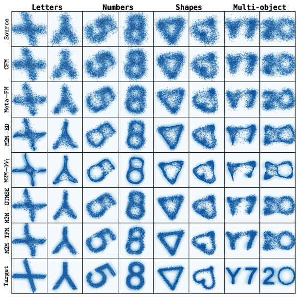
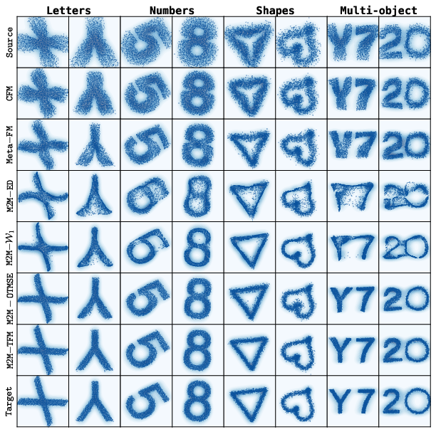
- Synthetic shapes (like moving point clouds that form letters or objects): The dynamic method was most accurate at reconstructing the target shapes.
- Systems where particles interact (like physics-inspired “McKean–Vlasov” systems): The methods handled distribution-dependent dynamics well—important because particles influence each other.
- Real biomedical data: Predicting how patient-derived mini-tumors (organoids) respond to treatments in colorectal cancer. The dynamic method performed strongly, showing practical medical relevance.
Why this matters:
- Many real systems—cells, crowds, particles, even collections of images—change as groups, not independently. Learning these group-to-group rules helps us predict outcomes more realistically.
What’s the impact?
- For science and medicine: These methods can help predict how entire cell populations will respond to drugs, supporting personalized treatment planning and experimental design.
- For physics and engineering: They can model complex, interacting systems where behavior depends on the whole population.
- For machine learning on sets: They show how transformers can act not just on sets, but as flexible “operators” that map one whole set-distribution to another, either in one step or as a smooth evolution.
In short, the paper introduces practical, powerful ways—especially the dynamic flow-based method—to learn how entire distributions evolve. This opens the door to better models for many problems where things move and change together.
Knowledge Gaps
Below is a single, focused list of concrete knowledge gaps, limitations, and open questions that remain unresolved by the paper. Each point is framed to be actionable for future research.
- Well-posedness of measure-dependent flows: What architectural or regularity conditions on transformer-parameterized vector fields guarantee existence, uniqueness, and stability of solutions to the measure-dependent ODE/continuity equation across training and test measures?
- Sample complexity and generalization bounds: What are the rates (in n paired measures, particle count N per measure, and dimension d) for generalization of static and dynamic M2M estimators to unseen measures, and how do they depend on attention depth/width and loss choice?
- Mass-splitting limitations: Deterministic pushforward maps fμ(x) cannot split mass for coincident or indistinguishable particles; when are stochastic Markov kernels (or randomized transformers) necessary, and how can they be learned scalably?
- Dependence on OT couplings: Both static OTMSE and dynamic flow matching rely on OT couplings (often mini-batch OT). How sensitive is training to coupling bias/noise, entropic regularization, and batch size, and can coupling-free (or coupling-robust) objectives be developed for M2M regression?
- Path design in flow matching: The method uses linear conditional paths φt(x,y). Do alternative paths (e.g., Gaussian, displacement interpolation under OT, Schrödinger bridges, stochastic flow matching) improve optimization, bias, or robustness for M2M?
- Computational scalability: Self-attention is O(N2) in particle count. What are the trade-offs and accuracy impacts of sparse/linear attention, token subsampling, or hierarchical/coarse-to-fine strategies for large measures (N ≫ 104)?
- High-dimensional performance: Distributional distances and OT estimation degrade in high d. How do static and dynamic methods perform and scale for very high-dimensional features (e.g., d ≳ 103–104), and what embedding or dimension-reduction strategies preserve M2M fidelity?
- Numerical integration errors: Dynamic inference uses Euler steps. How do step-size, adaptive ODE solvers, and integrator-in-the-loop training affect stability, accuracy, and long-horizon error accumulation in sequential M2M predictions?
- Structural constraint preservation: The learned flows are not constrained to be gradient fields or to obey known symmetries/conservation laws. How can one impose geometric/physical constraints (e.g., equivariances, conservation, support constraints) without sacrificing expressivity?
- Weighted and noisy measures: The methods assume uniform empirical measures. How to robustly handle weighted samples, measurement noise, and partial observability in practical datasets (e.g., varying cell capture rates)?
- Conditional operators with covariates: The formulation targets a fixed intervention operator. How to extend to conditional M2M operators f(μ | z) that adapt to patient metadata, dosage, time, or multi-intervention settings?
- Robustness to domain shift: How sensitive are models to batch effects, outliers, and shifts in the distribution over measures (e.g., new labs/sites, unseen patient populations), and what domain adaptation strategies work at the measure level?
- Identifiability and regularization: Multiple operators can fit finite paired measures. What inductive biases (e.g., Lipschitz, monotonicity, cycle consistency, invertibility) improve identifiability and prevent overfitting of M2M operators?
- Loss selection for static training: The paper compares MMD/ED/ Sinkhorn-W1/W2 but does not quantify bias–variance or gradient quality trade-offs. When does each loss yield better optimization and generalization, especially under limited sample sizes and high dimensions?
- Error control for mini-batch OT: Mini-batch OT couplings approximate global OT. What theoretical/empirical error bounds characterize their impact on learned operators and downstream performance?
- Baseline coverage: Comparisons omit several strong set-to-set operators (e.g., DeepSets with message passing, neural operators on measures, diffusion models over sets). A broader empirical study is needed to position M2M-TFM/static transformers w.r.t. these alternatives.
- Interpretability of learned operators: There is no analysis of attention/velocity-field structure. Can one extract interpretable interaction kernels, salient tokens, or conserved quantities from the learned M2M operators—especially in scientific domains?
- Uncertainty quantification: The methods output point estimates over measures. How to provide calibrated uncertainty over predicted measures (e.g., Bayesian transformers, ensembles, conformal calibration at the measure level)?
- Temporal consistency and semigroup properties: For multi-timepoint dynamics, do learned operators compose consistently (e.g., approximate semigroup)? What training objectives enforce temporal consistency across steps?
- Beyond Euclidean supports: Extension to measures on manifolds/graphs with appropriate equivariances and positional encodings remains open; what architectures and training protocols are needed?
- Static–dynamic equivalence and rates: Under what conditions does a dynamic transformer flow approximate any static M2M operator (and vice versa), and what are the approximation rates and stability trade-offs?
- Data requirements in real-world biology: What is the sensitivity of performance to the number of patients/measures, cells per measure, and inter-patient heterogeneity? How well do models generalize across laboratories and experimental protocols?
- Evaluation metrics at scale: ED and W1 are estimated from finite samples and can be high-variance in high d. What alternative or variance-reduced metrics better reflect measure-level fidelity and correlate with downstream utility?
- Training stability and regularization: Are there failure modes (e.g., mode collapse, over-smoothing, particle clumping)? Which regularizers (e.g., Jacobian/Lipschitz penalties, divergence controls, contrastive objectives) improve stability?
- Variable cardinality and partial overlap: While claimed “straightforward,” concrete algorithms and guarantees for handling widely varying support sizes and partial support overlaps between paired measures are not provided.
- Mixed data types and constraints: Many real datasets combine continuous features with categorical metadata or compositional constraints; how to incorporate mixed-type tokens and respect constraints within the M2M framework?
- Privacy and federated settings: Patient-level measures are sensitive. How to adapt M2M regression to federated/privacy-preserving training where measures cannot be pooled?
Practical Applications
Immediate Applications
Below are concrete ways the paper’s transformer-based measure-to-measure (M2M) regression methods (static and dynamic/TFM) can be used now, based on available tooling (e.g., transformers, GeomLoss/Sinkhorn, mini-batch OT, flow matching, standard DL frameworks).
- Healthcare/biotech: Rapid in‑vitro drug response prediction from single‑cell/organoid assays
- What: Train an M2M model on paired pre‑ vs post‑treatment single‑cell distributions to predict how a new patient’s pre‑treatment cell population will respond to a drug (as shown with colorectal cancer patient‑derived organoids).
- Tools/workflow: scRNA‑seq or imaging-based single‑cell profiles → preprocessing (batch correction/normalization) → compute couplings (mini‑batch OT) → train M2M‑TFM (dynamic) or static M2M with ED/MMD/Wasserstein loss → deploy inference as a pushforward operator for new patients.
- Assumptions/dependencies: same intervention/drug across training and test patients; high-quality paired datasets; careful handling of confounders; clinical use requires validation and regulatory approvals; computational budget for attention over large cell sets (may require sub-sampling/sparse attention).
- Biology research: Counterfactual prediction and imputation for perturbation screens
- What: Predict post‑perturbation distributions for conditions not measured (e.g., missing doses/timepoints/combos) from observed pre‑perturbation distributions.
- Tools/workflow: Integrate M2M‑TFM into existing single‑cell toolchains (e.g., Scanpy/Seurat pipelines); use mini‑batch OT or precomputed couplings; evaluate with ED/𝒲1/𝒲2 on holdout perturbations.
- Assumptions/dependencies: operator is stable across conditions in training; extrapolation beyond observed regimes can degrade; causal interpretations require additional design or instrumentation.
- Scientific computing: Fast surrogates for interacting particle systems
- What: Replace costly simulators (e.g., McKean–Vlasov SDEs) with learned M2M operators that map distributions across time, enabling rapid what‑if exploration.
- Tools/workflow: Generate paired measures along simulator trajectories → train M2M‑TFM on (μt → μt+Δt) → roll forward via ODE integration at inference.
- Assumptions/dependencies: training coverage must span dynamics of interest; numerical stability of the learned flow; generalization to new initial distributions depends on similarity to training data.
- Manufacturing/process control: Distribution-level quality prediction and drift monitoring
- What: Map incoming distributions of product features (e.g., particle sizes, shapes, tolerances) to expected output distributions after a process step; compare predicted vs observed to detect drift.
- Tools/workflow: Collect paired pre-/post‑step measurements as point clouds → train static M2M or M2M‑TFM → use predicted–observed distributional gaps (ED/𝒲1) for SPC alerts.
- Assumptions/dependencies: stationarity of the process; sufficient paired data; measurement noise and sensor bias handling.
- 3D vision/graphics: Point‑cloud denoising and de‑corruption
- What: Learn operators that reverse corruptions in point clouds (e.g., diffusion/kernel interactions), as demonstrated on 2D silhouette experiments—extendable to 3D scans.
- Tools/workflow: Train static M2M with Wasserstein/MMD loss or dynamic M2M‑TFM; integrate with point‑cloud pipelines (e.g., PCL/Open3D).
- Assumptions/dependencies: corruptions seen in training resemble test corruptions; compute cost scales with point count (may need downsampling).
- Finance/marketing analytics: Scenario‑conditioned distribution shift prediction
- What: Learn mappings from pre‑event distributions (returns, risk factors, customer transactions) to post‑event distributions for known interventions (policy, campaign, fee changes).
- Tools/workflow: Prepare paired event windows → train M2M operator per intervention → use for scenario testing and stress‑test libraries.
- Assumptions/dependencies: interventions consistent and repeatable; non‑stationarity and confounding must be addressed; compliance review for model risk.
- Energy/grid operations: Demand response distribution forecasting
- What: Map baseline load distributions across feeders/customers to post‑DR event distributions to plan capacity and incentives.
- Tools/workflow: Paired DR events data → M2M‑TFM for (pre‑event → post‑event) → portfolio‑level rollups and risk bounds via ED/𝒲1.
- Assumptions/dependencies: similar DR programs across training/test; privacy‑preserving aggregation may limit detail; seasonal/behavior changes can shift regimes.
- A/B testing and product analytics: Cohort‑level response mapping
- What: Predict changes in distributions of key metrics (e.g., session lengths, latency, spending) pre‑ and post‑launch or treatment.
- Tools/workflow: Build paired cohorts → train M2M operator → monitor predicted vs observed distributional effects to triage rollouts.
- Assumptions/dependencies: randomization/stratification to mitigate confounding; stable treatment effects across cohorts; compliance with privacy policies.
- Academic methods/benchmarks: General‑purpose M2M operator learning baselines
- What: Use the provided static and dynamic M2M approaches as baselines for new M2M datasets (e.g., multi‑measure objects, biological systems) and for theoretical studies of mean‑field transformers.
- Tools/workflow: Reproduce training with GeomLoss/Sinkhorn and mini‑batch OT; extend to different interpolation paths; publish standardized M2M regression benchmarks.
- Assumptions/dependencies: rigorous evaluation protocols (unseen measures), consistent coupling choices, and transparent hyperparameters.
Long‑Term Applications
These target larger‑scale deployment, new scientific or engineering integrations, or require additional research (e.g., safety, causal guarantees, real‑time constraints).
- Precision oncology clinical decision support
- What: Incorporate M2M‑TFM predictions into tumor boards to prioritize therapies from a patient’s baseline single‑cell profile and rapid in‑vitro testing.
- Potential products: Clinical software that takes a patient’s baseline assay and outputs distributional response forecasts and risk summaries.
- Assumptions/dependencies: prospective validation, trial evidence, regulatory clearance (FDA/EMA), robust handling of inter‑patient heterogeneity, end‑to‑end clinical workflows.
- Digital twins for tissues/organs and therapy planning
- What: Build distribution‑level simulators to forecast how cellular populations evolve under sequences of interventions (mono/combination therapies).
- Potential products: “Measure‑aware” digital twins interfacing with lab automation and EHRs; what‑if planners with uncertainty quantification.
- Assumptions/dependencies: longitudinal paired data, causal modeling for interventions, integration with mechanistic priors, governance for clinical safety.
- Swarm robotics and crowd management via distribution‑level controllers
- What: Learn measure‑dependent flow fields to guide swarms/crowds from initial to target state distributions under constraints.
- Potential products: Swarm controller design tools using M2M‑TFM with closed‑loop safety layers; simulation‑to‑real transfer frameworks.
- Assumptions/dependencies: real‑time inference and stability guarantees; robust perception-to-measure pipelines; safety certification.
- Public policy impact modeling on population distributions
- What: Map pre‑policy distributions (e.g., income, health, mobility) to post‑policy distributions to compare scenarios.
- Potential products: Policy sandbox platforms for distribution‑level impact assessments with fairness audits.
- Assumptions/dependencies: high‑quality paired observational/experimental data; causal identification strategies; ethical use and transparency.
- Grid‑scale control and market design under high renewables
- What: Design operator maps from fleet‑level baseline distributions (load/DERs) to controlled distributions under tariffs or dispatch policies.
- Potential products: Measure‑aware DR/DER orchestration; scenario engines for market rules.
- Assumptions/dependencies: integration with SCADA/AMI, privacy-preserving data aggregation, regulatory approval, resilience to rare events.
- Advanced manufacturing with closed‑loop distributional control
- What: Use M2M operators within MPC to steer product quality distributions to targets under varying inputs and disturbances.
- Potential products: Digital twins with distribution‑aware controllers; in‑line sensors feeding real‑time M2M predictions.
- Assumptions/dependencies: control‑theoretic guarantees for learned flows; sufficiently fast inference; robust sensors.
- Education and workforce development: Cohort‑level intervention planning
- What: Forecast distributions of learning outcomes under curriculum or policy changes to optimize interventions.
- Potential products: District dashboards with distributional forecasts and equity metrics.
- Assumptions/dependencies: ethically sourced paired data; bias/fairness safeguards; causal analysis beyond associational mapping.
- Foundation models for M2M operators
- What: Pretrain distribution‑to‑distribution transformers on large corpora of paired point‑cloud/measures (e.g., physics, bio, manufacturing) for cross‑domain transfer.
- Potential products: “M2M‑as‑a‑Service” APIs that adapt to task‑specific datasets with few‑shot finetuning.
- Assumptions/dependencies: standardization of M2M datasets, scalable attention (sparse/linear), privacy and IP frameworks.
- Physics‑informed and causality‑aware M2M flows
- What: Enforce conservation laws or incorporate causal structures to improve extrapolation and interpretability.
- Potential products: Domain‑constrained M2M libraries with PDE/stoichiometric constraints; tools to parse effects vs confounders.
- Assumptions/dependencies: hybrid training with simulators; identifiable interventions; new theory for constrained measure‑dependent flows.
Notes on feasibility across applications:
- Data requirements: Success hinges on curated paired measures representing the same operator (e.g., same drug/policy). Out‑of‑distribution interventions or unseen regimes reduce reliability.
- Computational costs: Attention scales roughly quadratically with point count; practical deployments may need subsampling, landmarking, or sparse attention.
- Identifiability: Purely associational training may not yield causal operators; mass‑splitting and non-uniqueness can arise without additional structure.
- Stability and safety: Dynamic flows require numerically stable integration and, in safety-critical settings, formal guarantees (e.g., Lyapunov‑based constraints).
- Governance: Fairness, privacy, and explainability are essential in domains like healthcare, finance, energy, and public policy.
Glossary
- Absolutely continuous (curve): A path of measures whose change is controlled in the Wasserstein metric, enabling differential equations on probability spaces. "a curve is absolutely continuous in the $2$-Wasserstein metric"
- Auto-regressive inference: Generating outputs by iteratively applying a model over multiple steps rather than in a single pass. "leveraging auto-regressive inference---iterating for multiple steps with the transformer to produce ---"
- Conditional Flow Matching (CFM): A training framework that regresses a vector field to match prescribed conditional paths between paired data points. "we extend Conditional Flow Matching (CFM) \citep{lipman2022flow, tong2023improving}"
- Continuity equation: A partial differential equation describing the evolution of probability measures under a velocity field. "satisfies a measure-dependent continuity equation of the form"
- Coupling (optimal transport plan): A joint distribution with specified marginals used to relate samples from two measures. "let denote a chosen coupling"
- Distribution alignment: Learning to match a distribution over measures (meta-distribution) rather than specific input–output measure pairs. "A second, distinct body of work addresses distribution alignment on "
- Empirical measure: A discrete probability measure placing equal mass on observed samples in a point cloud. "we represent by their empirical measure"
- Empirical ODE: An ordinary differential equation solved on the particles of a measure during inference. "solve the empirical ODE "
- Energy Distance (ED): A statistical distance between distributions based on expectations of pairwise distances. "energy distance (ED)"
- Euler integration: A simple numerical method to integrate ODEs by stepping forward with the current derivative. "(e.g., via Euler integration)"
- FitzHugh–Nagumo model: A dynamical system modeling excitable media (e.g., neurons) often used as a benchmark. "the Kuramoto model, Mean-Field Atlas, and the FitzHugh-Nagumo model"
- Flow map: The function that maps initial states to their states at time t under a time-dependent velocity field. "The natural geometric object underlying this viewpoint is the flow map on the ground space"
- Flow matching: A method that trains continuous-time generative or transport models by regressing to known or constructed velocities along paths. "Frameworks such as flow matching \citep{liu2022flow, lipman2022flow, tong2023improving, albergo2023stochastic} then provide a scalable route to training such models in practice."
- Kuramoto model: A model of coupled oscillators used to study synchronization phenomena. "the Kuramoto model, Mean-Field Atlas, and the FitzHugh-Nagumo model"
- Lipschitz continuous (operator): An operator whose outputs change at most proportionally to changes in the input measure, ensuring stability and representability. "who showed that Lipschitz continuous operators $$ can always be represented as~\eqref{eq:push}"</li> <li><strong>Markov kernel</strong>: A conditional probability mechanism mapping a point to a distribution, defining linear operators on measures. "induced by a Markov kernel $K$."</li> <li><strong>Markov operator</strong>: A linear operator on measures defined via a Markov kernel, transporting mass without measure-dependent nonlinearity. "A classical choice is a Markov (linear) operator $: \mathcal P(R^d) \to \mathcal P(R^d)$"</li> <li><strong>Maximum Mean Discrepancy (MMD)</strong>: A kernel-based distance between probability distributions used as a training loss. "the maximum mean discrepancy (MMD) distance"</li> <li><strong>McKean–Vlasov process</strong>: A stochastic/dynamical system whose evolution depends on the current distribution of the state (mean-field dynamics). "We evaluate our approaches for predicting the evolution of synthetic McKean-Vlasov processes"</li> <li><strong>Mean-field (structure)</strong>: A regime where interactions depend on aggregate statistics (the empirical distribution) rather than specific pairwise interactions. "leverages the natural measure-dependent and mean-field structure of transformers"</li> <li><strong>Mean-Field Atlas</strong>: A high-dimensional mean-field dynamical benchmark used for evaluating distribution-dependent modeling. "the Kuramoto model, Mean-Field Atlas, and the FitzHugh-Nagumo model"</li> <li><strong>Meta Flow Matching (Meta-FM)</strong>: A method that learns distribution-dependent vector fields using flow matching with a distributional encoder. "Meta Flow Matching (Meta-FM)"</li> <li><strong>Meta-distribution</strong>: A probability distribution over probability measures (distributions of datasets). "viewed as i.i.d.\ samples from an unknown meta-distribution on $\mathcal{P}(R^d)$"</li> <li><strong>Mini-batch OT</strong>: An approximation to optimal transport that computes couplings on mini-batches of samples for scalability. "via mini-batch OT"</li> <li><strong>Optimal transport (OT) map</strong>: A transport map that pushes one measure to another while minimizing a cost, often the squared Euclidean distance. "with the canonical choice being an optimal transport (OT) map"</li> <li><strong>Otto calculus</strong>: A formal Riemannian calculus on Wasserstein space enabling differential geometry of probability measures. "inspired by Otto calculus and the geometry of the Wasserstein space"</li> <li><strong>Permutation-equivariant</strong>: A property of functions on sets where permuting inputs results in the corresponding permutation of outputs. "using a permutation-equivariant velocity field, typically a transformer."</li> <li><strong>Pushforward (push-forward)</strong>: The transformation of a measure under a function, denoted $(f)_\sharp \mu$, moving mass via the map. "we consider a parametric class of pushforward operators"</li> <li><strong>Regression operator (on measures)</strong>: A mapping from input measures to output measures learned from paired distributions. "an unknown regression operator maps input measures to output measures."</li> <li><strong>Riemannian structure</strong>: A geometric structure allowing notions like gradients and geodesics; on Wasserstein space it arises from gradient fields. "yielding a Riemannian structure on $\mathcal P_2(R^d)$"</li> <li><strong>Score matching</strong>: A training paradigm that fits the score (gradient of log-density) to avoid hard distributional objectives. "this is precisely the difficulty that score matching was developed to circumvent"</li> <li><strong>Self-attention</strong>: A mechanism that computes interactions among tokens via learned query–key–value projections in transformers. "via the self-attention mechanism."</li> <li><strong>Sinkhorn algorithm</strong>: An entropic regularization method to efficiently approximate optimal transport and Wasserstein distances. "via the Sinkhorn algorithm \citep{cuturi2013sinkhorn}"</li> <li><strong>Tangent vector (in Wasserstein space)</strong>: An L2 vector field representing an instantaneous direction of change of a measure. "tangent vectors at a measure $\mu\chi:R^d\toR^d$"</li> <li><strong>Transformer Flow Matching (M2M-TFM)</strong>: The proposed method using time-dependent transformers to learn measure-dependent velocity fields via flow matching. "Transformer Flow Matching (M2M-TFM)"</li> <li><strong>Universal approximator</strong>: A model class capable of approximating any function in a target space to arbitrary accuracy under mild conditions. "deep transformers are universal approximators of M2M maps"</li> <li><strong>Velocity field</strong>: A vector field governing the instantaneous transport of points, which induces evolution of measures. "whose velocity field is itself distribution-dependent"</li> <li><strong>Wasserstein distance</strong>: A metric on probability measures based on optimal transport cost, with common variants $\mathcal{W}_1\mathcal{W}_2$. "the Wasserstein distances $\mathcal{W}_1, \mathcal{W}_2$"</li> <li><strong>Wasserstein Flow Matching (WFM)</strong>: A method that lifts flow matching to the space of probability measures using permutation-equivariant velocity fields. "Wasserstein Flow Matching (WFM)"</li> <li><strong>Wasserstein space</strong>: The metric space of probability measures endowed with the Wasserstein distance, often $\mathcal P_2(R^d)$. "the $2\mathcal P_2(R^d)$"