Large Scale Optimization of Disordered Hubbard Models through Tensor and Neural Networks

Abstract: We theoretically demonstrate a practical method for tuning randomly disordered 2D quantum-dot grids underlying spin qubit platforms using vision-based neural networks trained on tensor-network generated charge-stability data. We show that a simulatable local $3\times 3$ window already contains sufficient information to tune the central dot within a much larger array, thereby validating a sliding-window approach in which one tunes a local region and then translates that window across the lattice to calibrate a larger device. This avoids the computationally intractable necessity for obtaining the ground states for large systems with exponentially large Hilbert space. For the experimentally relevant case where only the on-site disorder is unknown, the neural network predicts the relevant parameters with very high fidelity in the $3\times 3$ setting [$R² &gt;0.99$], and after fine tuning on only a small number of larger-device samples, it retains high accuracy for the central dot of a $5\times 5$ plaquette [$R^2\approx 0.98$]. When all the dots parameters are treated as unknown, prediction of the on-site disorder remains robust [$R<sup>2&gt;0.9$ for both $3\times 3$ and $5\times 5$], although the remaining parameters are substantially more difficult to infer from the same charge-stability data. This shows that the most practically important disorder parameter for tuning can still be inferred reliably even in the fully disordered setting for the computationally difficult 5x5 arrays.

• The paper presents a sliding-window approach combining tensor-network simulations and advanced neural network architectures for scalable parameter inference.
• Using charge-stability diagrams as inputs, the method robustly predicts on-site disorder with high accuracy (R² > 0.98 for 3×3 and 5×5 windows).
• The approach offers practical implications for automated tuning of quantum dot arrays while laying the foundation for improved inference of other Hubbard model parameters.

Large Scale Optimization of Disordered Hubbard Models Using Tensor and Neural Networks

Motivation and Context

The calibration and optimization of large arrays of semiconductor quantum dots for spin qubit applications remains a major technical challenge due to the inherent disorder present in realistic devices. The extended 2D Hubbard model provides an accurate framework to describe the underlying physics, but its exponentially growing Hilbert space renders direct parameter inference and device-scale simulation computationally intractable. This paper develops a scalable strategy leveraging tensor-network simulated measurement data and vision-based neural networks to infer local Hubbard-model parameters from experimentally accessible charge-stability diagrams. The work addresses both computational and physical locality constraints by employing a sliding-window approach, where a neural network is trained on simulated windows (e.g., $3\times 3$ regions) and then used to tune the central dot as this window moves across the larger lattice.

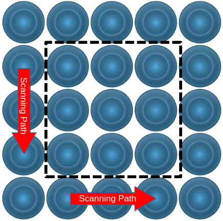
Figure 1: Sliding-window process for tuning large quantum dot arrays via transferable local neural models.

Physical Model and Simulation Methodology

The studied system consists of a two-dimensional grid of quantum dots modeled by the extended Hubbard Hamiltonian: $$H = -\sum_{\langle i,j\rangle, \sigma} t_{ij}( c_{i\sigma}^\dagger c_{j\sigma} + h.c. ) - \sum_i \epsilon_i n_i + \sum_{\langle i,j\rangle} V_{ij} n_i n_j + \sum_i \frac{U_i}{2} n_i(n_i-1)$$ where sites are indexed by $i$, $t_{ij}$ is the nearest-neighbor hopping amplitude, $\epsilon_i$ is the site disorder potential, $V_{ij}$ is the inter-site Coulomb repulsion, and $U_i$ is the on-site repulsion. The task is to infer ${t_{ij}, V_{ij}, U_{i}, \epsilon_{i}}$ from measured occupations, typically at low temperature.

Tensor-network techniques, specifically MPS and DMRG algorithms implemented in ITensor, enable ground-state simulations for window sizes up to $5\times5$ that are otherwise prohibitive for exact diagonalization. The 2D lattice is mapped to a 1D chain by snaking connections to minimize long-range interaction and reduce bond dimension requirements.

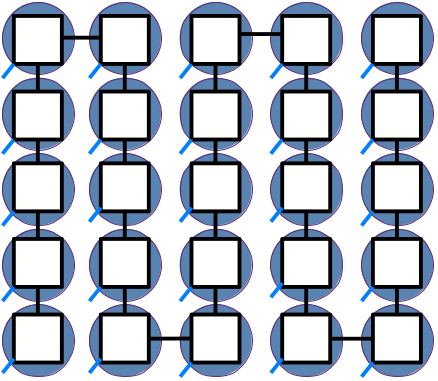
Figure 2: Tensor network diagram of MPS representation with snaking site order to minimize interaction length.

Neural Network Architecture and Training

The charge-stability measurements required for parameter inference are simulated for various disorder realizations. Each realization produces a tensor $X$ of site occupation values for a grid of chemical potentials, forming the input to the neural network. The architecture is a 3D convolutional model incorporating squeeze-and-excitation layers for global contextual information, followed by adaptive pooling and dense layers. Distinct networks are trained for each parameter, as the visual features associated with $$H = -\sum_{\langle i,j\rangle, \sigma} t_{ij}( c_{i\sigma}^\dagger c_{j\sigma} + h.c. ) - \sum_i \epsilon_i n_i + \sum_{\langle i,j\rangle} V_{ij} n_i n_j + \sum_i \frac{U_i}{2} n_i(n_i-1)$$0, $$H = -\sum_{\langle i,j\rangle, \sigma} t_{ij}( c_{i\sigma}^\dagger c_{j\sigma} + h.c. ) - \sum_i \epsilon_i n_i + \sum_{\langle i,j\rangle} V_{ij} n_i n_j + \sum_i \frac{U_i}{2} n_i(n_i-1)$$1, $$H = -\sum_{\langle i,j\rangle, \sigma} t_{ij}( c_{i\sigma}^\dagger c_{j\sigma} + h.c. ) - \sum_i \epsilon_i n_i + \sum_{\langle i,j\rangle} V_{ij} n_i n_j + \sum_i \frac{U_i}{2} n_i(n_i-1)$$2, and $$H = -\sum_{\langle i,j\rangle, \sigma} t_{ij}( c_{i\sigma}^\dagger c_{j\sigma} + h.c. ) - \sum_i \epsilon_i n_i + \sum_{\langle i,j\rangle} V_{ij} n_i n_j + \sum_i \frac{U_i}{2} n_i(n_i-1)$$3 are not generally identical.

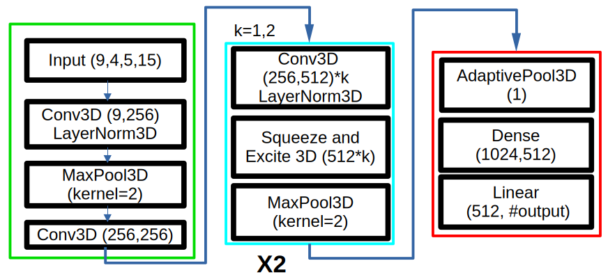
Figure 3: Neural network architecture composed of convolutional, squeeze-and-excitation, and dense layers.

The training protocol uses 6500 disorder realizations for $$H = -\sum_{\langle i,j\rangle, \sigma} t_{ij}( c_{i\sigma}^\dagger c_{j\sigma} + h.c. ) - \sum_i \epsilon_i n_i + \sum_{\langle i,j\rangle} V_{ij} n_i n_j + \sum_i \frac{U_i}{2} n_i(n_i-1)$$4 windows, with a small number (200) of $$H = -\sum_{\langle i,j\rangle, \sigma} t_{ij}( c_{i\sigma}^\dagger c_{j\sigma} + h.c. ) - \sum_i \epsilon_i n_i + \sum_{\langle i,j\rangle} V_{ij} n_i n_j + \sum_i \frac{U_i}{2} n_i(n_i-1)$$5 samples for fine-tuning transfer performance. Early stopping and learning rate decay schedules are chosen based on validation performance across both window sizes.

Results

On-site Disorder Only

For the scenario where only $$H = -\sum_{\langle i,j\rangle, \sigma} t_{ij}( c_{i\sigma}^\dagger c_{j\sigma} + h.c. ) - \sum_i \epsilon_i n_i + \sum_{\langle i,j\rangle} V_{ij} n_i n_j + \sum_i \frac{U_i}{2} n_i(n_i-1)$$6 is unknown (all other parameters fixed), the neural network predicts the central dot disorder potential with high fidelity:

• $$H = -\sum_{\langle i,j\rangle, \sigma} t_{ij}( c_{i\sigma}^\dagger c_{j\sigma} + h.c. ) - \sum_i \epsilon_i n_i + \sum_{\langle i,j\rangle} V_{ij} n_i n_j + \sum_i \frac{U_i}{2} n_i(n_i-1)$$7 window: $$H = -\sum_{\langle i,j\rangle, \sigma} t_{ij}( c_{i\sigma}^\dagger c_{j\sigma} + h.c. ) - \sum_i \epsilon_i n_i + \sum_{\langle i,j\rangle} V_{ij} n_i n_j + \sum_i \frac{U_i}{2} n_i(n_i-1)$$8, $$H = -\sum_{\langle i,j\rangle, \sigma} t_{ij}( c_{i\sigma}^\dagger c_{j\sigma} + h.c. ) - \sum_i \epsilon_i n_i + \sum_{\langle i,j\rangle} V_{ij} n_i n_j + \sum_i \frac{U_i}{2} n_i(n_i-1)$$9
• $i$0 window after $i$1 fine-tuning: $i$2, $i$3

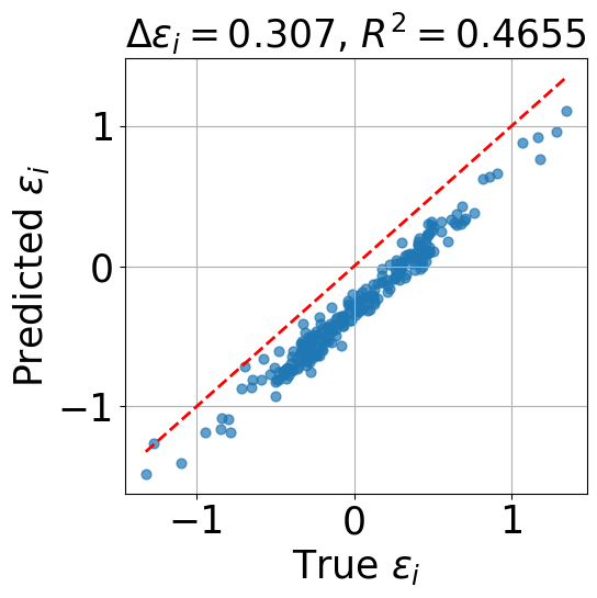
Figure 4: Prediction vs. expected $i$4 in $i$5 arrays using network trained only on $i$6 data (no fine-tuning); demonstrates a residual linear shift.

Fine-tuning on a small set of larger-window samples corrects a residual linear offset and achieves robust inference for the central dot in larger arrays.

All Parameters Unknown

When all parameters are treated as unknown, the neural network continues to infer $i$7 robustly for both window sizes:

• $i$8 window: $i$9, $t_{ij}$0
• $t_{ij}$1 window: $t_{ij}$2, $t_{ij}$3

Prediction accuracy for $t_{ij}$4, $t_{ij}$5, and $t_{ij}$6 is substantially lower ($t_{ij}$7 in range $t_{ij}$8), likely due to limited charge-stability diagram point density and insufficient training sample diversity.

Input Representation

Charge-stability diagrams, the direct neural network inputs, are constructed as occupation matrices indexed by chemical potential and nearest-neighbor link direction for each site.

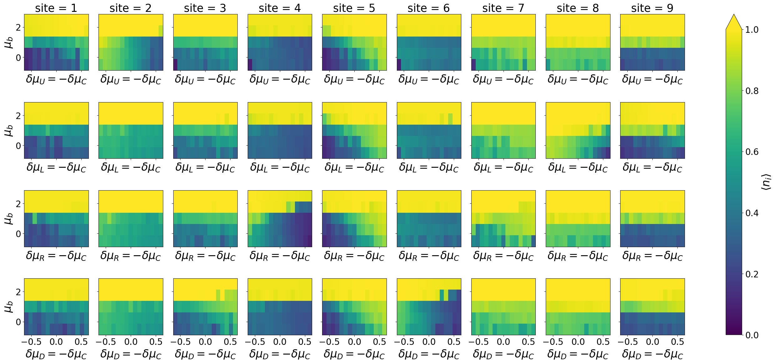
Figure 5: Example charge-stability diagram, input basis for neural network parameter inference.

Practical and Theoretical Implications

The strong fidelity of $t_{ij}$9 predictions confirms that the most critical disorder parameter for device calibration can be inferred locally, supporting scalable automated tuning in experimental settings. The sliding-window training approach, validated by robust transfer to $\epsilon_i$0 arrays with minimal additional fine-tuning, is compatible with large-scale architectures and modular device manufacturing. While predictions of $\epsilon_i$1, $\epsilon_i$2, and $\epsilon_i$3 remain suboptimal, the methodology provides a foundation for future improvements, including enhanced measurement resolution, increased sample counts, and more advanced neural architectures. The extension of this framework to larger windows is tractable and offers diminishing returns for system-size corrections.

From a theoretical perspective, this demonstrates that locality in charge-stability measurements is sufficient for reliable parameter inference in strongly interacting disordered systems, bypassing the need for full-array simulation and circumventing exponential complexity. The successful application of vision-based neural networks, trained on high-fidelity tensor-network data, suggests scalability for future quantum-dot device platforms and lays ground for similar strategies in other lattice quantum electronic systems.

Figure 1: Sliding-window process for large-scale tuning

Figure 3: Schematic of neural architecture for charge-stability inference

Figure 2: MPS tensor-network mapping for 2D lattice simulation

Figure 5: Charge-stability diagram input basis

Figure 4: Predicted vs. expected $\epsilon_i$4 in $\epsilon_i$5 arrays, linear offset without fine-tuning

Conclusion

This work establishes a practical methodology for scalable optimization of disordered Hubbard-model quantum-dot lattices, combining tensor-network simulation for training data generation with convolutional neural networks for local parameter inference. The sliding-window approach achieves highly accurate prediction of on-site disorder potentials for both small and moderately large arrays, substantiating its suitability for automated device calibration and control. While inference of additional Hubbard parameters remains challenging, the methodology provides a versatile platform for further algorithmic and hardware advancements in quantum device automation. Future directions include increased measurement resolution, larger window training, and transferability to experimental charge-stability data.

(2604.18711)