A sub-asymptotic model for bivariate threshold exceedances

Abstract: Extreme value theory offers a statistical framework for quantifying the risk of rare events, with the generalized Pareto (GP) distribution providing the canonical limit model for univariate threshold exceedances. In many applications, however, extremes are intrinsically multivariate, requiring models that capture both marginal tail behaviours and joint extremal dependencies. Under asymptotic dependence, the multivariate GP distribution represents a suitable modelling family, but when asymptotic independence arises, sub-asymptotic models are needed. In this work, we propose and study a flexible sub-asymptotic parametric class to model bivariate threshold exceedances. Our new model accommodates a broad range of tail dependence behaviours and contains the standardised multivariate GP distribution as a limiting case while retaining margins that converge to univariate GP tails. Our formulation allows extremal dependence to evolve naturally with the marginal parameters on the original data scale, facilitating direct computation and interpretation of failure probabilities. Model inference is done via a likelihood-free neural Bayes estimation approach, with tailored prior specifications. An extensive simulation study and an application to Belgian rainfall extremes illustrate the estimation framework and the flexibility of the model.

• The paper proposes the sBGP model that unifies asymptotic independence and dependence in bivariate threshold exceedances to improve joint tail modeling.
• It employs an exponential-gamma framework with a tunable weight parameter to smoothly interpolate between weak and strong tail dependence regimes.
• The methodology leverages a neural Bayes estimator for likelihood-free inference, achieving robust parameter estimation in sub-asymptotic settings.

A Sub-Asymptotic Model for Bivariate Threshold Exceedances

Introduction and Theoretical Motivation

The proposed model, the sub-asymptotic bivariate GP (sBGP) distribution, addresses the modeling of bivariate threshold exceedances, particularly accommodating the transition between asymptotic dependence (AD) and asymptotic independence (AI), which is not suitably handled by the standard multivariate GP (MGP) distribution. Traditional MGPs are valid under AD but lack flexibility in the AI regime, where joint extremes decay more rapidly. The sBGP model fills this gap by furnishing a mechanism that unifies AI and AD within one framework, capturing a much broader spectrum of extremal dependence regimes.

The core idea is to build on the exponential-gamma stochastic representation foundational in univariate GP theory and to generalize this to the bivariate context. The construction preserves Pareto tails in the margins while allowing a smooth interpolation between weak and strong joint tail dependence, introducing the weight parameter $w$ to tune shared vs. independent contributions in the model. The resulting structure allows direct inference on the data's native scale and supports likelihood-free parameter estimation, leveraging neural Bayes estimation (NBE).

Model Construction and Extremal Dependence Structure

The sBGP model is given by: $$Y = \left(\beta_1 \left( \frac{w E + (1-w) E_1}{G + G_1} - S_1 \right), \beta_2 \left( \frac{w E + (1-w) E_2}{G + G_2} - S_2 \right)\right)^\top,$$ where $E, E_1, E_2$ are independent exponential, $G, G_1, G_2$ are independent gamma random variables, and $(S_1, S_2)$ is a non-negative shift with L-shaped support. The parameters $(\alpha, \alpha_1, \alpha_2)$ govern the tail regime, $(\beta_1, \beta_2)$ control marginal scaling, $w$ mediates the mixture between shared and idiosyncratic exponential components, and $\sigma_T$ (in the $S$ construction) captures sub-asymptotic dependence.

The marginal distributions are heavy-tailed (regular variation of order $$Y = \left(\beta_1 \left( \frac{w E + (1-w) E_1}{G + G_1} - S_1 \right), \beta_2 \left( \frac{w E + (1-w) E_2}{G + G_2} - S_2 \right)\right)^\top,$$0) and converge to GP marginals. The table below summarizes the asymptotic regimes as a function of the gamma shape parameters and weight $$Y = \left(\beta_1 \left( \frac{w E + (1-w) E_1}{G + G_1} - S_1 \right), \beta_2 \left( \frac{w E + (1-w) E_2}{G + G_2} - S_2 \right)\right)^\top,$$1:

Regime (Gamma parameters)	$$Y = \left(\beta_1 \left( \frac{w E + (1-w) E_1}{G + G_1} - S_1 \right), \beta_2 \left( \frac{w E + (1-w) E_2}{G + G_2} - S_2 \right)\right)^\top,$$2	$$Y = \left(\beta_1 \left( \frac{w E + (1-w) E_1}{G + G_1} - S_1 \right), \beta_2 \left( \frac{w E + (1-w) E_2}{G + G_2} - S_2 \right)\right)^\top,$$3	$$Y = \left(\beta_1 \left( \frac{w E + (1-w) E_1}{G + G_1} - S_1 \right), \beta_2 \left( \frac{w E + (1-w) E_2}{G + G_2} - S_2 \right)\right)^\top,$$4
$$Y = \left(\beta_1 \left( \frac{w E + (1-w) E_1}{G + G_1} - S_1 \right), \beta_2 \left( \frac{w E + (1-w) E_2}{G + G_2} - S_2 \right)\right)^\top,$$5	$$Y = \left(\beta_1 \left( \frac{w E + (1-w) E_1}{G + G_1} - S_1 \right), \beta_2 \left( \frac{w E + (1-w) E_2}{G + G_2} - S_2 \right)\right)^\top,$$6, $$Y = \left(\beta_1 \left( \frac{w E + (1-w) E_1}{G + G_1} - S_1 \right), \beta_2 \left( \frac{w E + (1-w) E_2}{G + G_2} - S_2 \right)\right)^\top,$$7	Same $$Y = \left(\beta_1 \left( \frac{w E + (1-w) E_1}{G + G_1} - S_1 \right), \beta_2 \left( \frac{w E + (1-w) E_2}{G + G_2} - S_2 \right)\right)^\top,$$8, $$Y = \left(\beta_1 \left( \frac{w E + (1-w) E_1}{G + G_1} - S_1 \right), \beta_2 \left( \frac{w E + (1-w) E_2}{G + G_2} - S_2 \right)\right)^\top,$$9	Same
$E, E_1, E_2$0	$E, E_1, E_2$1	$E, E_1, E_2$2	$E, E_1, E_2$3

The weight $E, E_1, E_2$4 drives the strength of tail dependence in AD: as $E, E_1, E_2$5 increases, so does $E, E_1, E_2$6 (the tail dependence coefficient). In the AI regime, $E, E_1, E_2$7 becomes irrelevant asymptotically, but is critical for finite thresholds.

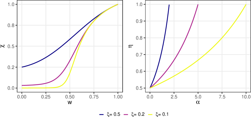
Figure 1: Limiting tail dependence coefficients $E, E_1, E_2$8 (left) and $E, E_1, E_2$9 (right) as functions of the weight $G, G_1, G_2$0.

Notably, the limiting MGP arises as a boundary case (all gamma shapes $G, G_1, G_2$1, $G, G_1, G_2$2), and the model's L-shaped support matches the canonical region for threshold exceedance modeling.

Sub-Asymptotic Features and Diagnostics

In finite sample applications, convergence to the asymptotic regime may be slow. The sBGP framework provides access to sub-asymptotic diagnostics, with dependence assessed by the full $G, G_1, G_2$3 and $G, G_1, G_2$4 curves (for quantile level $G, G_1, G_2$5), not just their limiting values.

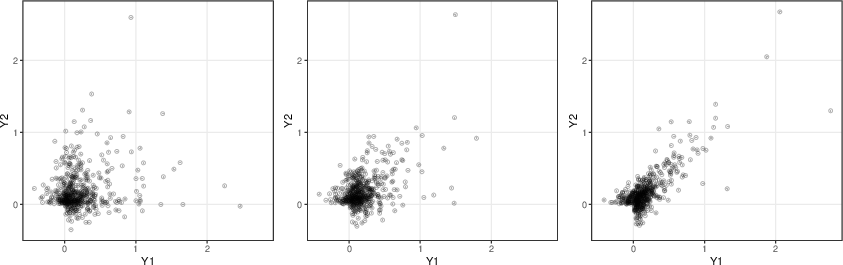
Figure 2: Scatterplots from sBGP model with identical $G, G_1, G_2$6 but varying $G, G_1, G_2$7; sub-asymptotic dependence clearly differs.

The figure above demonstrates that samples with the same residual tail dependence can display vastly different intermediate dependence structures as $G, G_1, G_2$8 varies—an effect invisible to asymptotic summaries. Model assessment thus focuses on the empirical estimation of these curves, obtained via simulation, to capture the true range of extremal co-movement observed in finite samples.

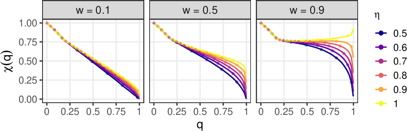
Figure 3: Empirical $G, G_1, G_2$9 curves for the sBGP model: $(S_1, S_2)$0 modulates the sub-asymptotic regime even at identical $(S_1, S_2)$1.

Parameter Estimation: Neural Bayes Estimator (NBE)

Classical likelihood-based inference is intractable for the sBGP model due to the complex joint structure. Instead, a likelihood-free approach is employed, specifically the neural Bayes estimator [sainsbury-dale_likelihood-free_2024]. The NBE is trained on large ensembles of simulated datasets covering a broad prior over the parameter space, automatically learning informative summary statistics for estimation.

The estimation can be stabilized by a penalization term acting on the deviation of model-based residual tail dependence $(S_1, S_2)$2 from a robust empirical estimator. The prior and neural architecture are carefully designed to ensure good coverage over both AI and AD regimes. In simulations, the estimator demonstrates good point accuracy and well-calibrated uncertainty intervals across a broad spectrum of dependence scenarios.

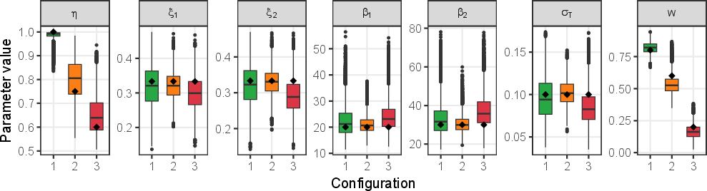
Figure 4: Boxplots for parameter estimates under multiple tail dependence regimes show high estimation accuracy and appropriate uncertainty quantification.

Empirical Application: Belgian Rainfall Extremes

The sBGP model is applied to weekly precipitation maxima from the ERA5 dataset over Belgium. Exceedances are defined relative to high quantiles, and the model is fitted pairwise (e.g., Brussels–Nivelles and Ostend–Spa), demonstrating the capacity to recover both the marginal tails and extremal dependence structure.

Spatial fields of parameter estimates reveal coherent geographic patterns: dependence decays with distance, and the residual tail dependence $(S_1, S_2)$3 and sub-asymptotic weight $(S_1, S_2)$4 both decrease further from the reference site.

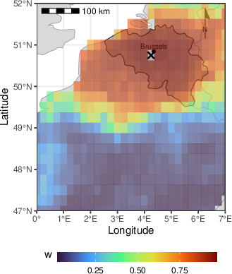
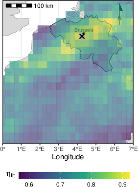
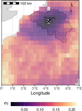
Figure 5: Spatial fields of $(S_1, S_2)$5, $(S_1, S_2)$6, and $(S_1, S_2)$7 for sBGP fits between Brussels and neighboring grid points.

For selected pairs, QQ plots of marginal fits indicate that the sBGP model reproduces the entire upper tail well. Comparison of empirical and fitted $(S_1, S_2)$8 curves shows that the sBGP captures both strong and weak dependence regimes. Particularly, for the more distant (cross-regional) pair, the model correctly identifies weak upper tail dependence, which standard MGP fitting cannot recover.

Benchmarking Against Multivariate GP

Fitting both the sBGP and standard MGP distributions at a high threshold reveals the consequences of model selection: MGP enforces asymptotic dependence and threshold stability, leading to systematic biases and poorer marginal fits when threshold stability is not observed. The sBGP, by contrast, replicates the empirically observed weakening of dependence in the upper tail and maintains better fit for failure probabilities relevant to risk calculations.

Implications and Future Extensions

Practically, the sBGP provides a tractable, interpretable, and computationally efficient approach for multivariate extremes, crucial for applications where risk quantification relies on realistic joint tail estimates (e.g., in hydrology or finance). Theoretically, it closes the gap in multivariate exceedance modeling across the full AI–AD spectrum and highlights the importance of sub-asymptotic diagnostics in practical statistics.

For dimensionalities $(S_1, S_2)$9, generalization is straightforward in principle (with appropriate combinatorics of shared/individual gamma components), but complexity grows rapidly; parsimonious structures are recommended to maintain identifiability and interpretability.

Conclusion

The sub-asymptotic bivariate GP model offers substantial advances over classical approaches, enabling flexible modeling and inference of joint threshold exceedances across the full range of extremal dependence regimes. The integration with neural Bayes estimators provides robust, likelihood-free inference, scalable to large sample sizes and complex dependence structures. This model constitutes a significant augmentation of the EVT toolkit for realistic multivariate risk assessment.

For complete technical details, see "A sub-asymptotic model for bivariate threshold exceedances" (2604.12405).