More Vertices of the Tristochastic Polytope

Abstract: The $n\times n$ doubly stochastic matrices constitute a polytope in $\mathbb{R}<sup>{n<sup>2}$, and by Birkhoff's theorem, its vertex set coincides with the set of order-$n$ permutation matrices.\ A tristochastic array is an $n \times n\times n$ array of nonnegative reals, where each row, column, and shaft sums to one. These arrays constitute a polytope $Δ_n$ in $\mathbb{R}<sup>{n<sup>3}$. In analogy, it is easy to see that each of the $L_n$ order-$n$ Latin squares is a vertex of $Δ_n$, but in contrast to Birkhoff's theorem, Latin squares form a vanishingly small subset of $Δ_n$'s vertex set. We show here that $Δ_n$ has at least $L_n<sup>{2-o(1)}$ vertices.

• The paper improves the vertex lower bound for Δₙ to n^(2-o(1)n²) by constructing a large family of vertices with 0 and 1/2 entries.
• The paper introduces a multi-stage, layered construction that leverages Hamiltonian cycles and perfect matchings to enforce connectivity and non-bipartiteness in the support graphs.
• The paper’s method sharply distinguishes the combinatorial structure of tristochastic polytopes from the Birkhoff polytope, suggesting new directions in high-dimensional extreme point enumeration.

Structural and Combinatorial Analysis of the Tristochastic Polytope

Introduction and Theoretical Background

The tristochastic polytope $\Delta_n$—the set of all $n\times n\times n$ arrays of non-negative real numbers with each line (row, column, shaft) summing to unity—serves as a high-dimensional analog of the classical Birkhoff polytope for doubly stochastic matrices. By Birkhoff’s theorem, the vertex set of the Birkhoff polytope is in bijection with permutation matrices. For the tristochastic case, the Latin squares of order $n$ (arrays with precisely one $1$ in each line, zeros elsewhere) are vertices of $\Delta_n$, but previous work established that Latin squares constitute only a negligible fraction of all vertices as $n$ grows (e.g., $L_n = ((1+o(1))n/e^2)^{n^2}$ [van Lint & Wilson]). The prior lower bound on the vertex count in $\Delta_n$ was $n^{(\frac{3}{2} - o(1)) n^2}$ [linial2014vertices], while the present work achieves a significant improvement.

Summary of Main Results

The principal achievement is a new lower bound: the vertex count of $\Delta_n$ is at least $n\times n\times n$0. This is accomplished by explicitly constructing a large new family of vertices, relying on careful combinatorial techniques and high-dimensional regularity arguments. The constructed vertices use only $n\times n\times n$1 and $n\times n\times n$2 entries—exhibiting support patterns that go far beyond Latin squares—and each array is verified to be an extreme point via a graph-theoretic characterization based on connectivity and non-bipartiteness of an associated $n\times n\times n$3 graph.

Construction Framework and Key Stages

The generation of vertices proceeds in five tightly orchestrated stages, built layer-by-layer:

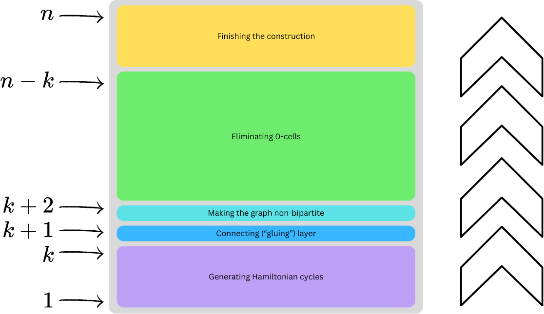
Figure 1: The construction has five stages, progressing from the bottom-up; each stage incrementally builds complexity and removes regularity constraints to guarantee vertexhood and maximize count.

1. Stage 1 (Layers 1 to $n\times n\times n$4): The $n\times n\times n$5 layers are partitioned into $n\times n\times n$6 subarrays. Each layer comprises two disjoint Hamiltonian cycles of $n\times n\times n$7 entries, one in each quadrant, ensuring each line is covered exactly twice. Diagonal minors are explicitly reserved and filled with "standard cycles."

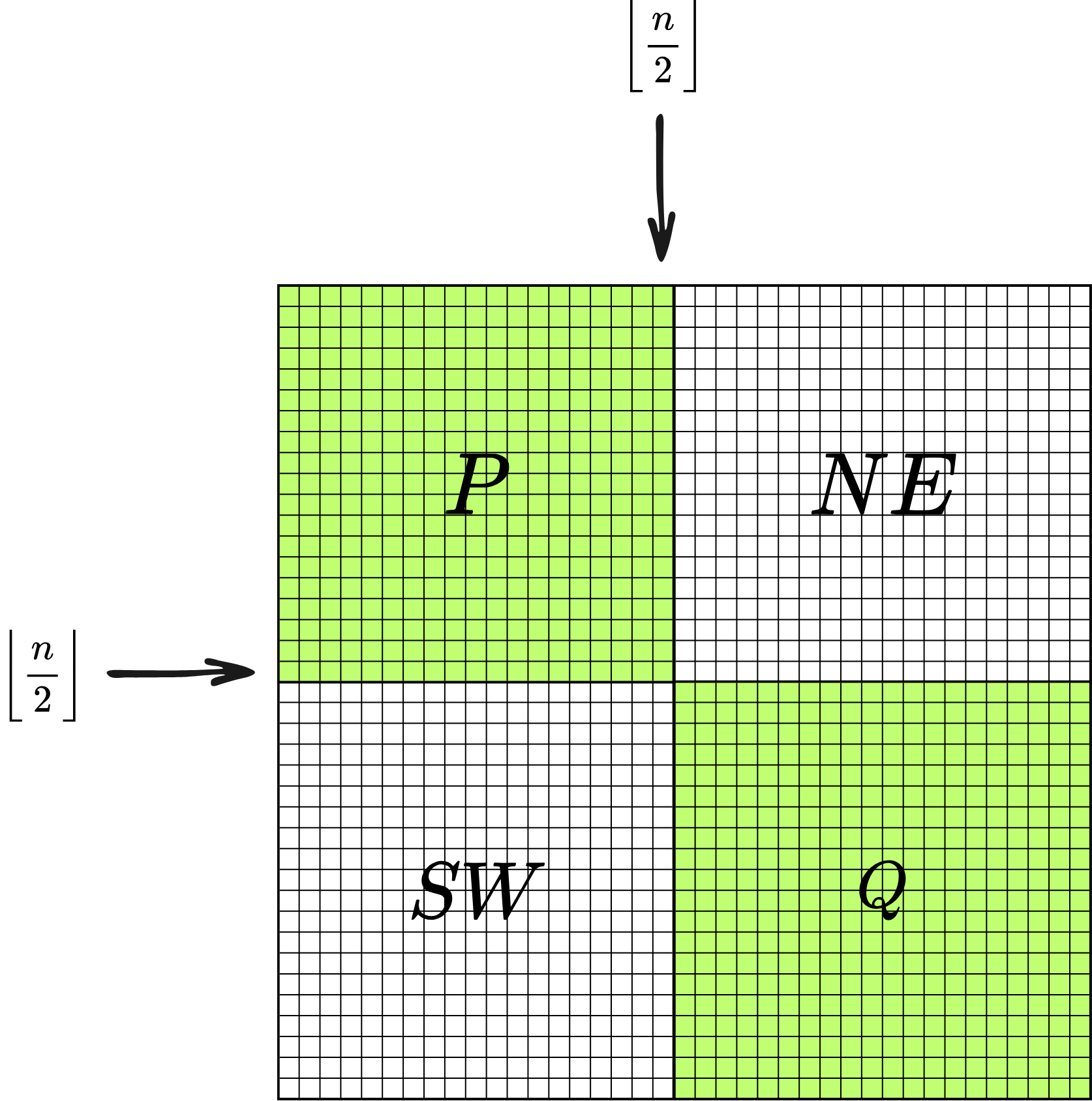
Figure 2: $n\times n\times n$8 is split into NW ($n\times n\times n$9), SE ($n$0), NE, and SW subarrays, isolating regions for independent cycle insertion.

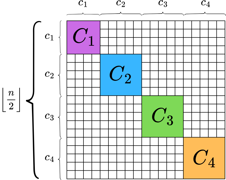
Figure 3: Diagonal minors $n$1 in $n$2 align with $n$3 layers, laying groundwork for support diversity and later non-bipartiteness.

Construction of $n$4 is illustrated, with the placement of standard cycles in each $n$5 minor:

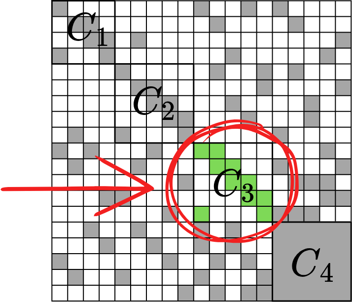
Figure 4: Standard cycle insertion into a minor $n$6 of a layer, with prior and reserved minors demarcated.

Cycles are accommodated in subarrays $n$7—removing influence from prior minors and walls—for which Hamiltonicity is guaranteed via Moon–Moser-type degree bounds:

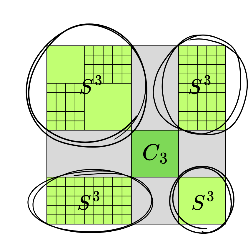
Figure 5: The subarray $n$8 (light green), avoiding already filled walls/minors, is the domain for a new Hamiltonian cycle in layer 3.

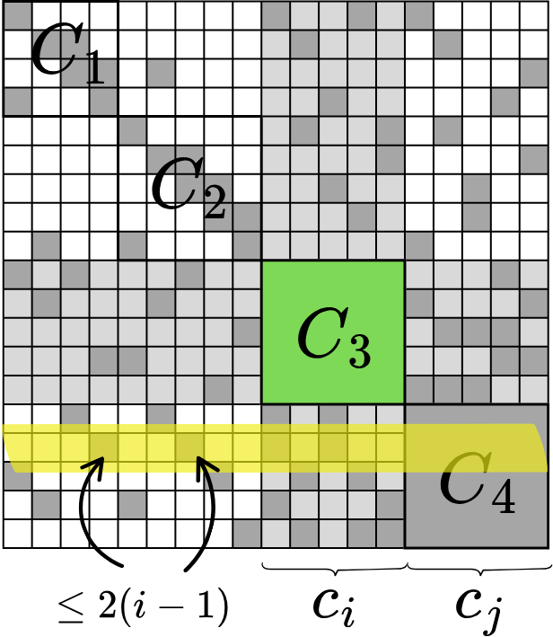
Figure 6: Lower bounding degrees in $n$9 via enumeration of zeros in $1$0 is crucial for existence of Hamiltonian cycles.

Each constructed layer merges its two disjoint cycles (minor and complement) using a local switching argument, ensuring the resulting structure remains within the $1$1 class and meets the required connectivity:

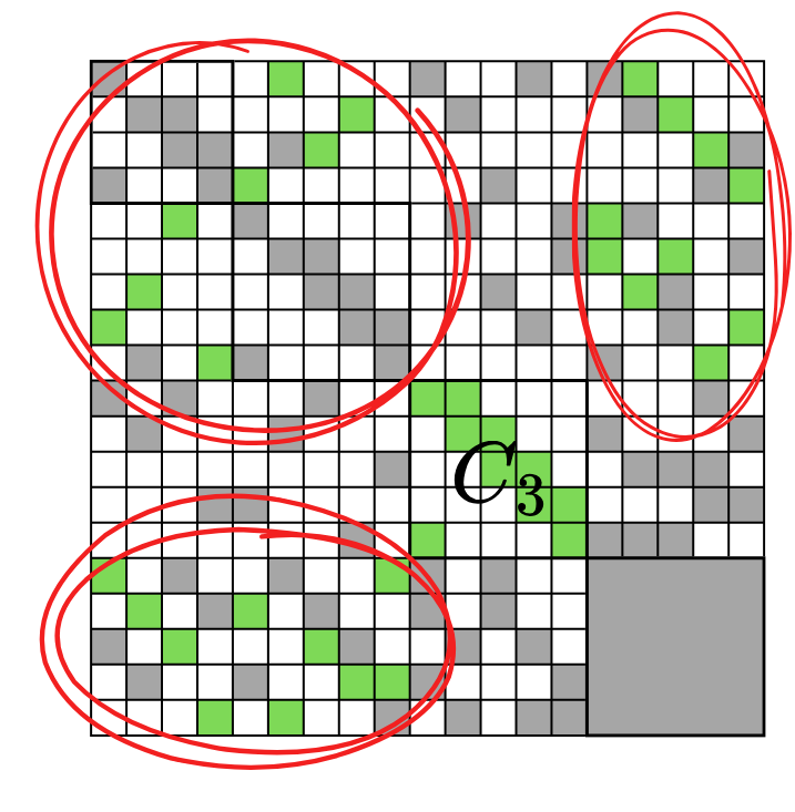
Figure 7: Merging operation overlays the newly inserted cycle in $1$2 and the current minor.

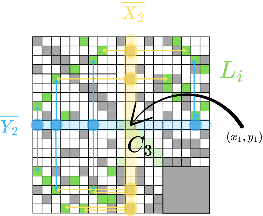
Figure 8: Identification of swap candidates between a minor and the cycle for merging involves careful exclusion of dependent positions.

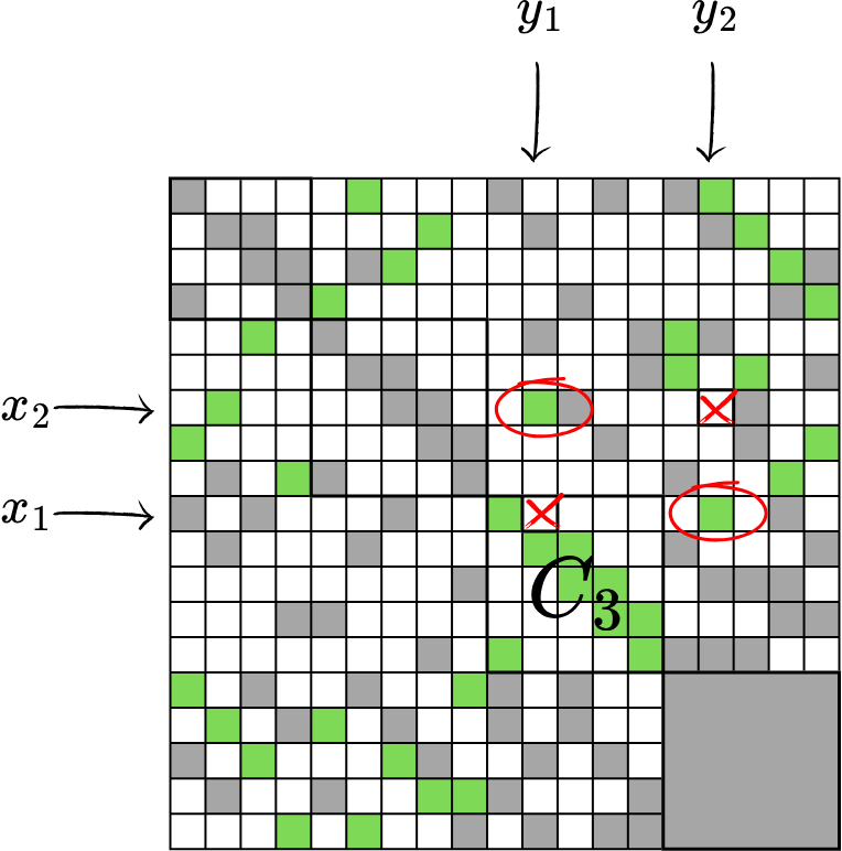
Figure 9: The actual swap operation guaranteeing a single connected Hamiltonian cycle in the layer.

2. Stage 2 (Layer $1$3): This layer "glues" all lower cycles into a single connected structure through a specifically constructed cycle covering diagonals and auxiliary slots.

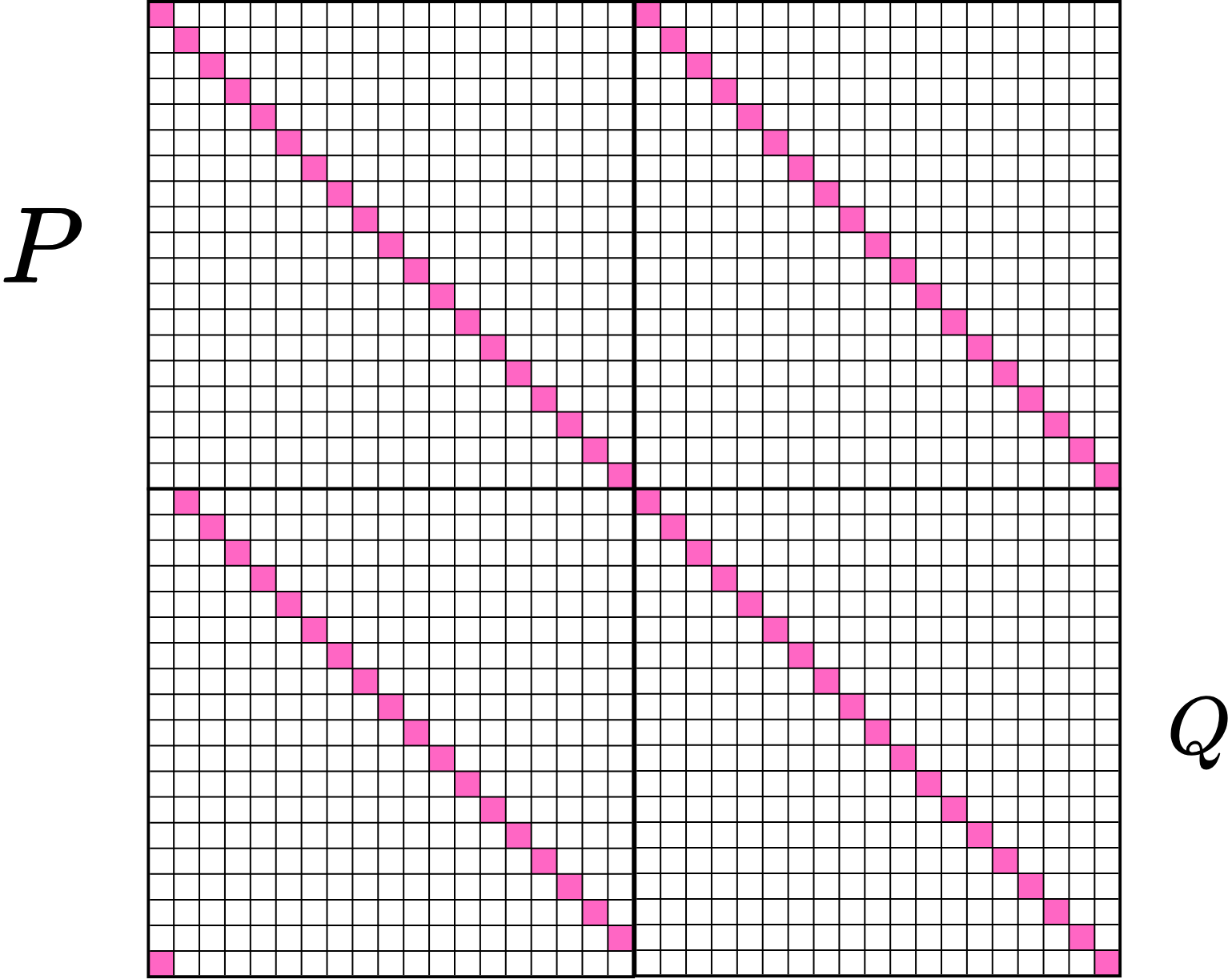
Figure 10: When $1$4 is even, the connectivity layer aligns cycles across all quadrants using both diagonal and off-diagonal support.

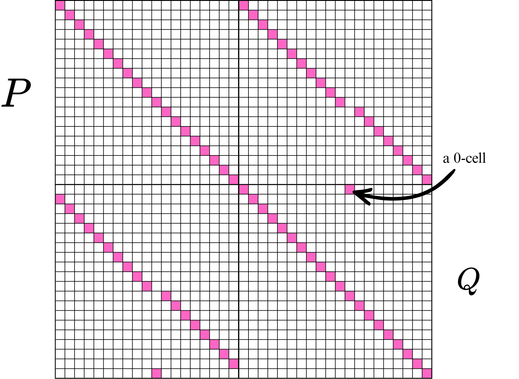
Figure 11: For odd $1$5, the construction requires additional support in $1$6 to ensure the cycle closes.

3. Stage 3 (Layer $1$7): Enforces non-bipartiteness in $1$8 via insertion of two disjoint perfect matchings: one in the graph induced by $1$9-cells ("bi-chromatic," forced by coloring inherited from lower layers), and another in the $\Delta_n$0-support. The interplay of edge colorings guarantees an odd cycle.

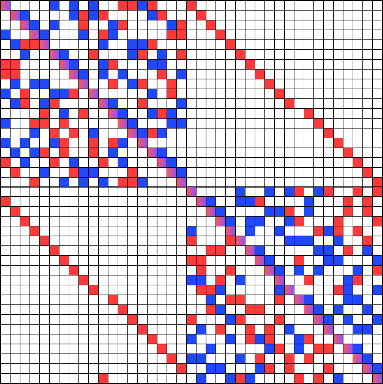
Figure 12: The induced $\Delta_n$1-coloring of $\Delta_n$2 prior to permutation placement.

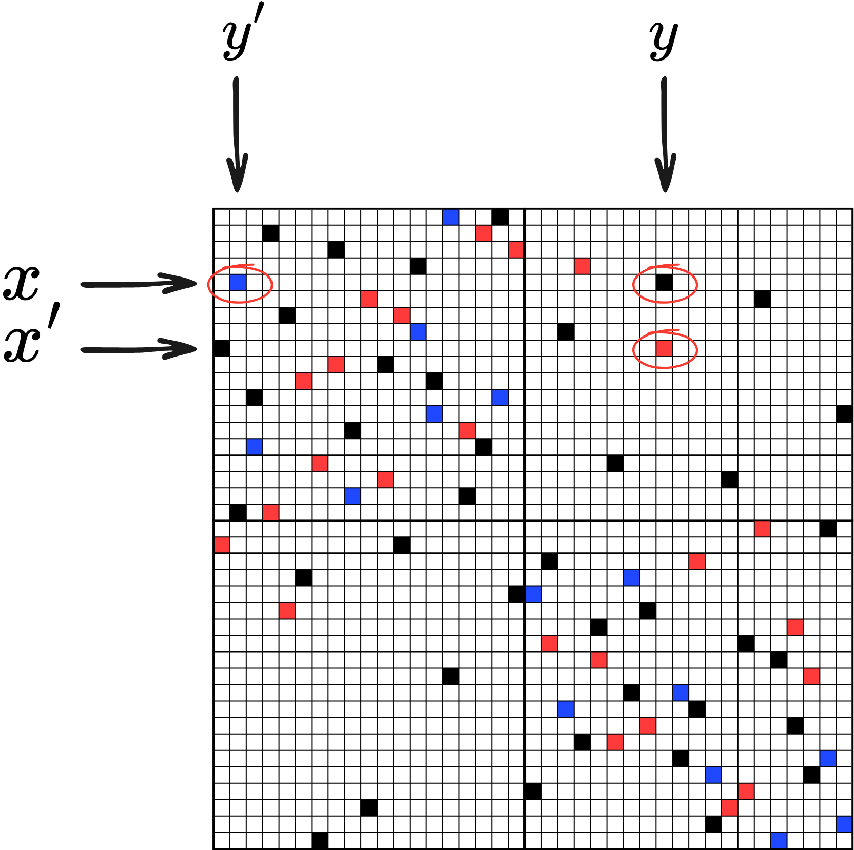
Figure 13: Layer $\Delta_n$3, showing interleaving bi-colored permutations of $\Delta_n$4 cells (red/blue) and a permutation of $\Delta_n$5-cells (black) to force non-bipartiteness in $\Delta_n$6.

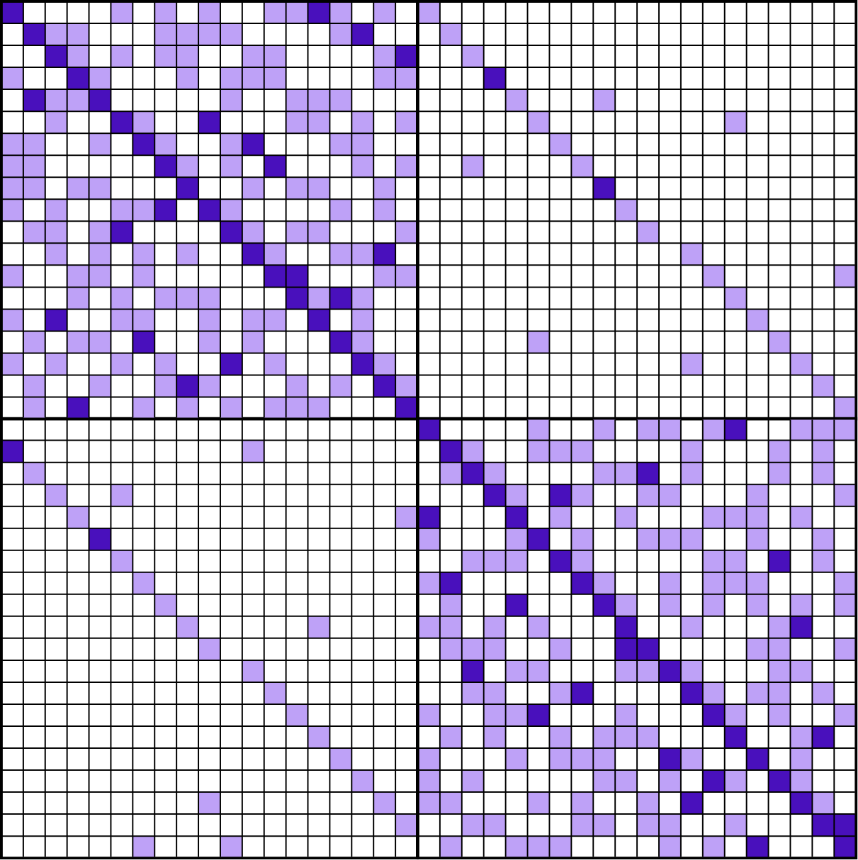
Figure 14: Construction of slice $\Delta_n$7 visualized, where purple colors denote growing support for $\Delta_n$8-cells and $\Delta_n$9-cells as the structure progresses.

1. Stage 4 (Layers $n$0 through $n$1): Successive elimination of all $n$2-cells by placing two perfect matchings per layer, maintaining regularity and incrementally growing the support.
2. Stage 5 (Layers $n$3 through $n$4): Final elimination of all remaining $n$5-cells by iteratively inserting disjoint perfect matchings (now both in the same support graph).

Quantitative Lower Bounds and Enumeration

The new vertex count lower bound is substantiated through detailed enumeration of constructional degrees of freedom:

• Stage 1: Each of the $n$6 cycles across $n$7 layers offers at least $n$8 choices, by leveraging the Kahn–Cuckler exponential bound on Hamiltonian cycles in regular bipartite graphs.
• Stage 4: The perfect matchings count contributes $n$9.
• Stage 5: The final completions contribute another factor of $L_n = ((1+o(1))n/e^2)^{n^2}$0.

Multiplying across all stages yields the final exponent of $L_n = ((1+o(1))n/e^2)^{n^2}$1 in $L_n = ((1+o(1))n/e^2)^{n^2}$2.

Numerical Exploration: Support Patterns

Random sampling (with nonuniformity caveats) reveals that as $L_n = ((1+o(1))n/e^2)^{n^2}$3 increases, the line-supports of sampled vertices diversify and observed support sizes per line often cluster at $L_n = ((1+o(1))n/e^2)^{n^2}$4 or $L_n = ((1+o(1))n/e^2)^{n^2}$5. The histograms highlight this phenomenon over a range of $L_n = ((1+o(1))n/e^2)^{n^2}$6.

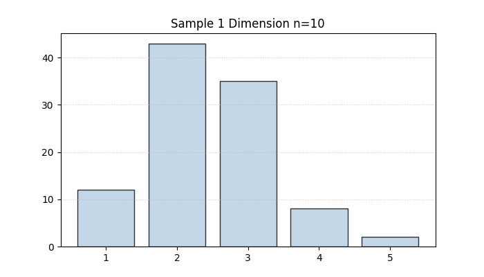
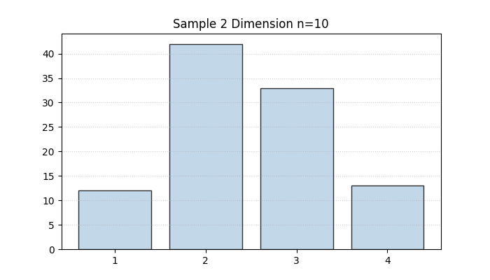
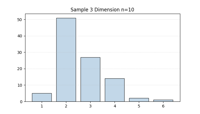
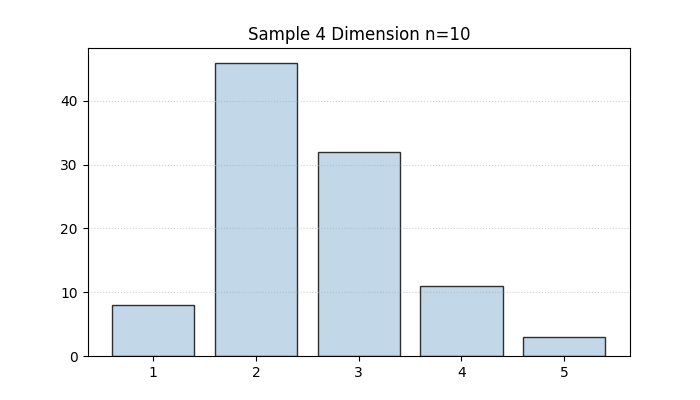
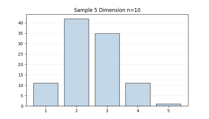
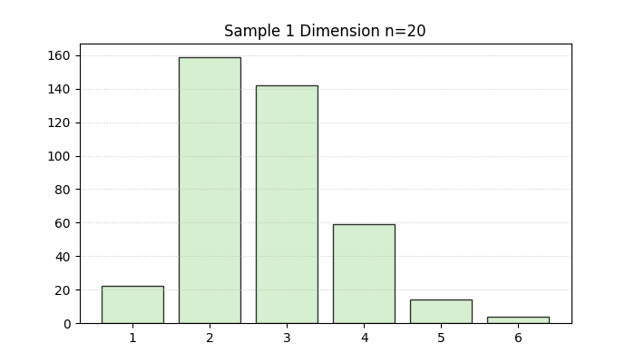
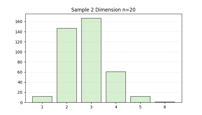
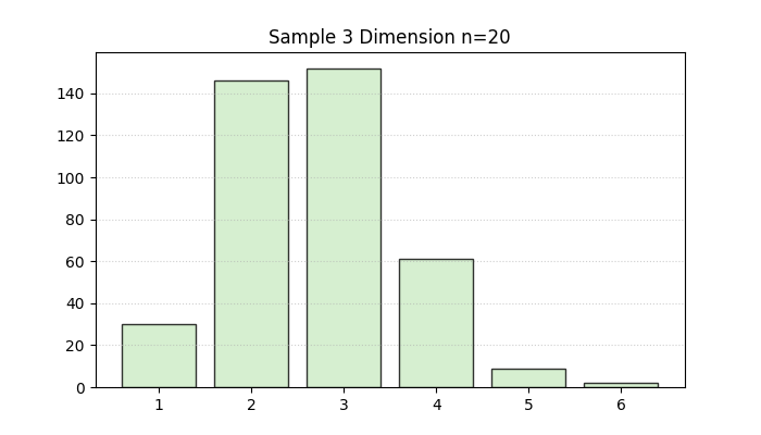
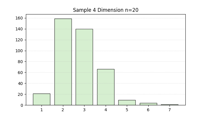
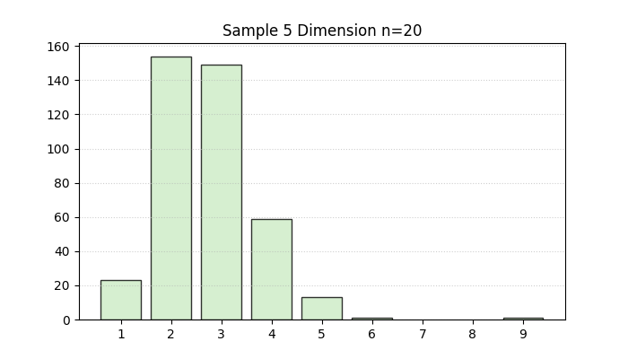
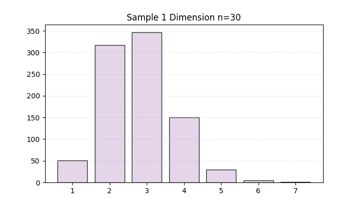
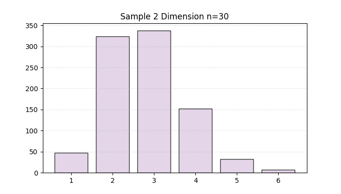
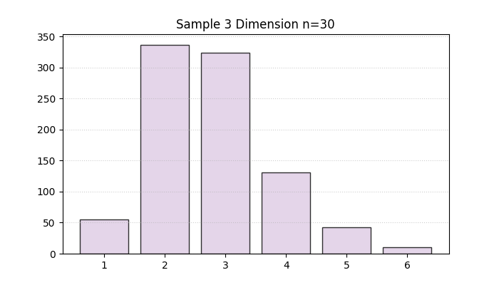
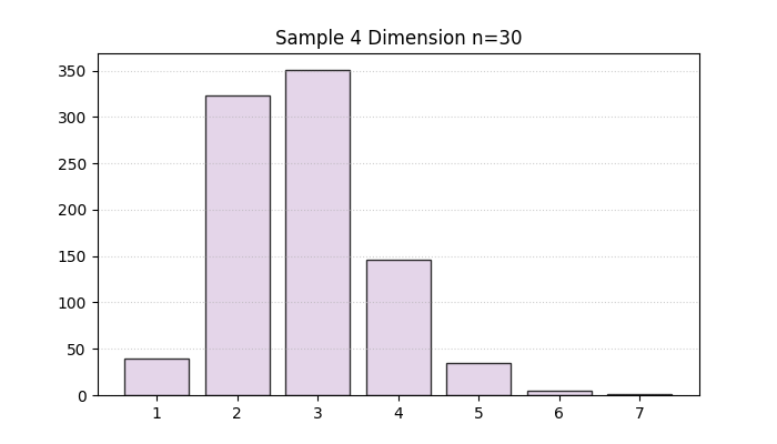
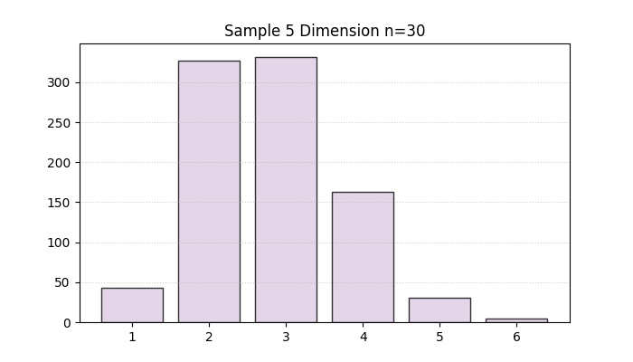
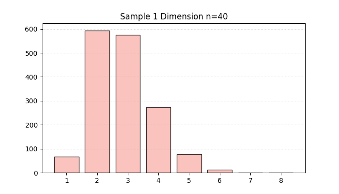
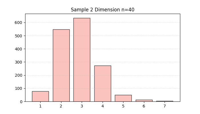
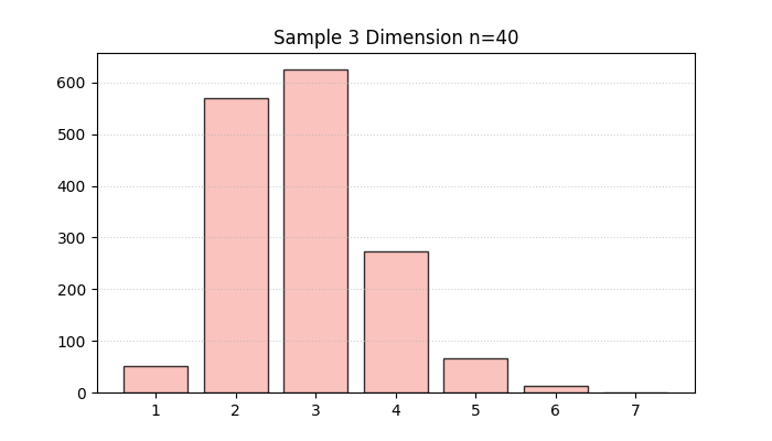
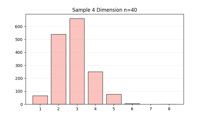
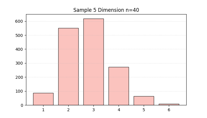
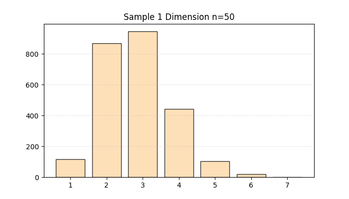
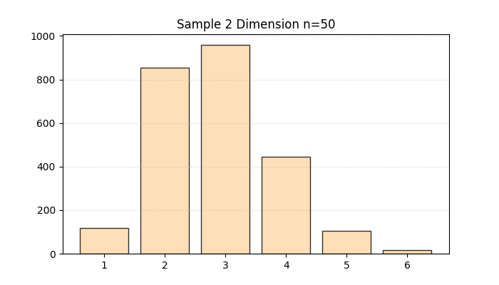
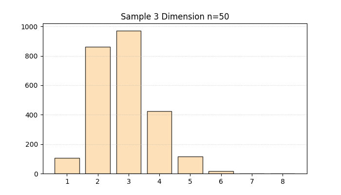
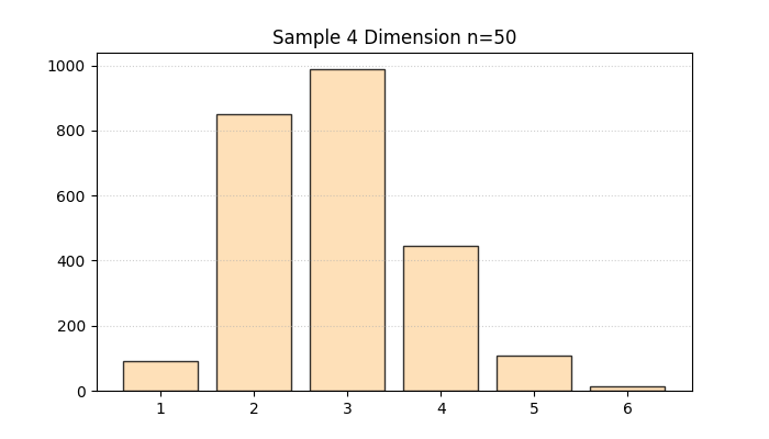
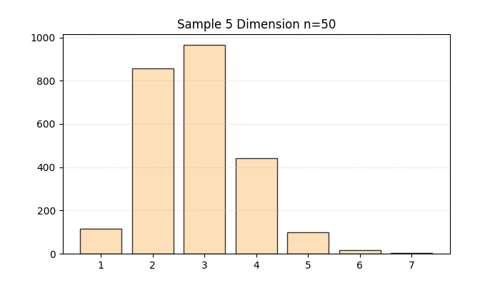
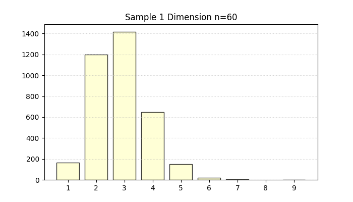
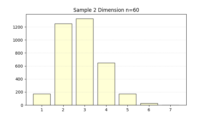
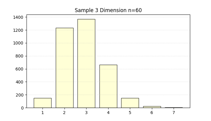
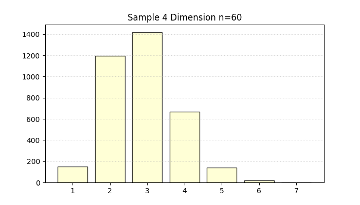
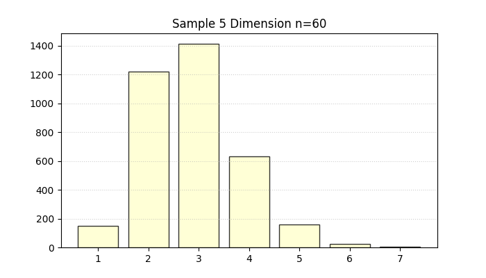
Figure 15: Empirical histograms of row support sizes in sampled tri-stochastic vertices for $L_n = ((1+o(1))n/e^2)^{n^2}$7 through $L_n = ((1+o(1))n/e^2)^{n^2}$8, indicating a prevalence of small support but extensive variation.

Implications and Future Directions

This result substantially closes the exponential gap between known lower (now $L_n = ((1+o(1))n/e^2)^{n^2}$9) and upper ($\Delta_n$0, by uniqueness of support) bounds on the vertex count of the tristochastic polytope. It also sharply distinguishes the structure of $\Delta_n$1 from that of the Birkhoff polytope: the typical vertex is not a Latin square; it is highly structured but combinatorially far richer, with support and values not accessible via classical permutation/Latin square arguments.

The methodology—monolithic layered constructions enforcing connectivity/non-bipartiteness in support graphs—demonstrates a flexible paradigm for extreme point enumeration in high-dimensional stochastic polytopes. With open questions about the maximum support size per line and the detailed structure of higher-dimensional faces, the combinatorics of tristochastic and multistochastic polytopes remains a highly fertile research area, with potential implications for random array models, extremal combinatorics, and high-dimensional probability.

Conclusion

This work yields a near-sharp exponential lower bound on the vertex set size of the tristochastic polytope, vastly expanding the known landscape beyond Latin squares. The use of high-dimensional Hamiltonian cycle mixing, support-graph non-bipartiteness, and regularity arguments establishes a template for further combinatorial investigations into extreme points of structured polytopes. Future research may pursue both tighter bounds and a more refined classification of the geometry and combinatorics of such high-dimensional stochastic structures.

(2604.09290)