A Regularized Auxiliary Variable (RAV) Approach for Gradient Flows

Abstract: In this paper, we propose a regularized auxiliary variable (RAV) approach and construct accurate and robust time-discrete schemes for a large class of gradient flows. By introducing an auxiliary variable $r=0$ and constructing an auxiliary equation that naturally fits into the energy relation, the numerical solution $r^{n+1}$ of the auxiliary variable is corrected at each time step to preserve consistency with the original system. The developed RAV scheme satisfies unconditional energy stability with respect to the original variables, and in certain cases the original energy law can be directly recovered. Furthermore, we obtain a uniform bound on the norm of the numerical solution, which allows us to establish the optimal error estimate in $L^\infty(0,T;H^2)$ for the second-order scheme without any restriction on the time step. We present ample numerical results, including comparisons with the scalar auxiliary variable (SAV) approach, to demonstrate the accuracy and effectiveness of the proposed RAV approach.

• The paper presents a RAV scheme that enforces the auxiliary-variable relation with analytic corrections, eliminating drift and ensuring unconditional energy stability.
• It demonstrates second-order convergence and optimal error estimates in strong norms, surpassing the limitations of traditional SAV methods.
• Numerical experiments on phase-field and interfacial models confirm the method’s efficiency and robustness for complex dissipative PDEs.

A Regularized Auxiliary Variable (RAV) Approach for Gradient Flows

Introduction and Motivation

The paper introduces a Regularized Auxiliary Variable (RAV) approach for constructing accurate and robust time-discrete schemes for a broad family of gradient flows, including those arising in interfacial dynamics, phase-field models, and related dissipative PDE contexts. The method's core innovation is the introduction of an auxiliary variable—carefully coupled to the energy relation of the original flow—and its regularized treatment, ensuring enhanced consistency with the underlying dynamics relative to existing auxiliary variable formulations such as the Scalar Auxiliary Variable (SAV) method.

Unlike SAV, which often suffers from numerical drift in enforcing the discrete-algebraic relation between the auxiliary variable and the state variable, RAV enforces this relationship at each step using analytic correction strategies inspired by regularization methodologies for DAEs. This results in unconditional energy stability and optimal error estimates in strong norms (e.g., $L^\infty(0,T;H^2)$ for second-order schemes) without further temporal resolution constraints.

Theoretical Construction of the RAV Scheme

The standard gradient flow is generated from a free energy functional, with the evolution expressed in the variational gradient descent direction. The SAV methodology introduces a scalar auxiliary variable that augments the PDE, allowing one to construct unconditionally energy-stable, efficient linear schemes. Yet, the SAV discretization, by taking time derivatives of algebraic relations, introduces index reduction errors and drift from the original algebraic constraint. The RAV scheme resolves this by more tightly enforcing $r=0$ (the auxiliary constraint) through analytic correction at each time step.

The construction proceeds as follows:

• For gradient flow of a single scalar (e.g., the Cahn-Hilliard equation), a time-dependent auxiliary variable $r$ is introduced.
• A regularization equation is formulated to ensure that the deviation between the time derivative form and the algebraic definition is dissipative and consistently driven to zero.
• The RAV scheme consists of a coupled time-discrete system for the primary and auxiliary variable, where analytic correction aligns the auxiliary variable at every step to its original algebraic value.
• The modified energy used in stability proofs tightly bounds the deviation between the primary variable and the auxiliary.

The step-by-step treatment, summarized below, demonstrates the analytic, correction-based update of $r$ (ensuring $r^{n+1}$ stays at zero unless numerical dissipation pushes it negative, in which case it is strictly controlled):

• Compute $\phi^{n+1}$ from the linearized, semi-implicit system.
• Update $Q^{n+1}$, summarizing energy drift and dissipation, to determine the correction required for the auxiliary variable.
• Apply analytic projection to enforce regularity in the auxiliary equation.
• Deduce from the discrete energy law the uniform bounds on the numerical solution, crucial for strong norm error estimates.

Energy Stability and Error Analysis

The RAV approach achieves unconditional energy stability for both the original and the modified energy laws. Specifically:

• For $Q^{n+1}\geq 0$, RAV yields decay according to the original energy functional, matching the theoretical PDE dissipation.
• For $Q^{n+1}<0$, the method corrects the auxiliary variable to avoid artificial growth in energy, strictly capping the possible numerical error.

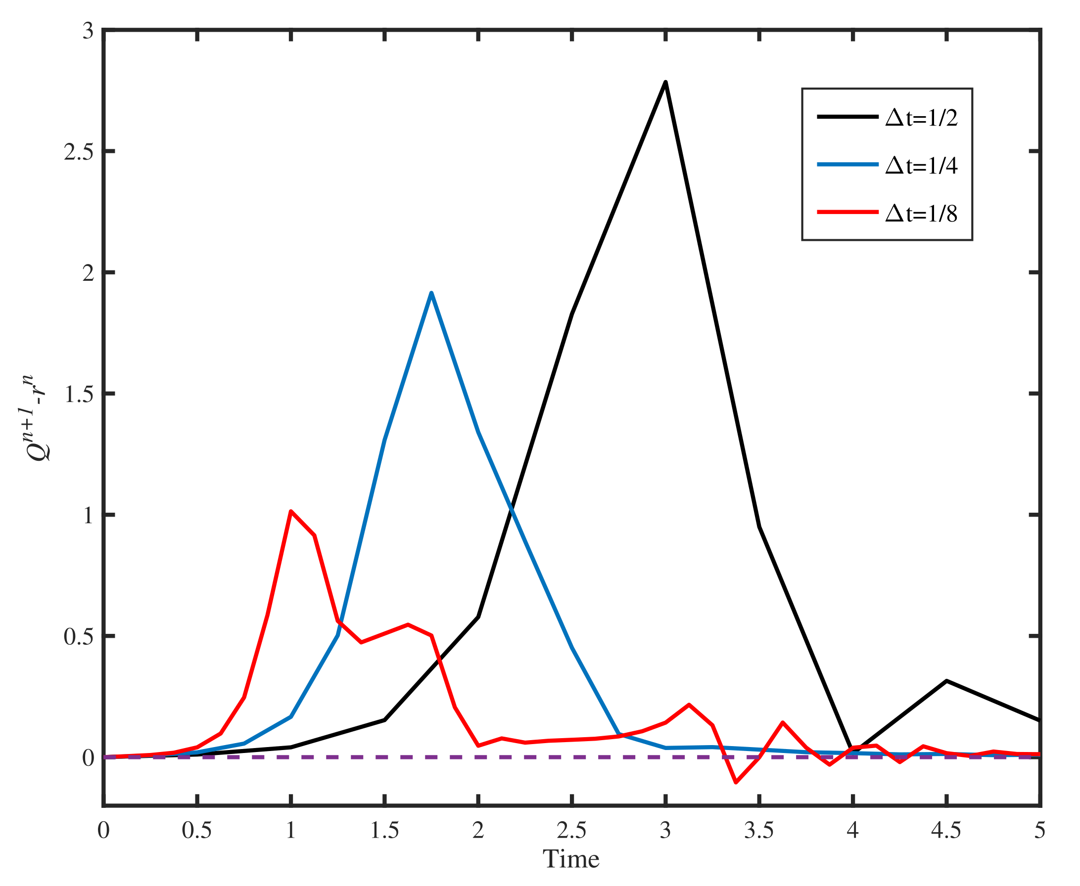
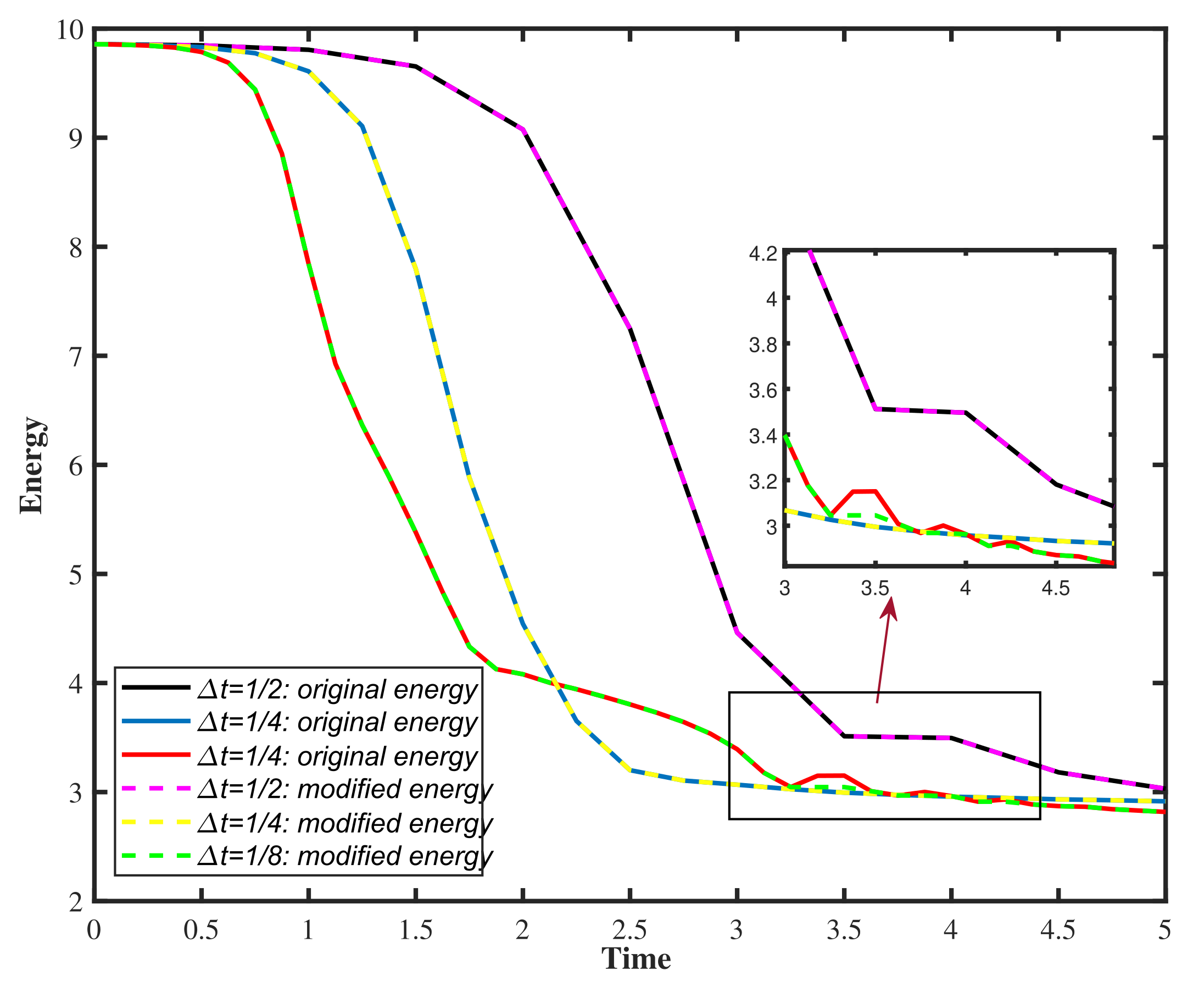
Figure 1: Evolution of total energy for the RAV scheme with different time steps.

Analytically, the approach provides uniform $L^\infty(0,T;H^2)$ bounds, and the error analysis demonstrates second-order convergence without restriction on the time step—improving upon previous auxiliary variable schemes that required step-size constraints to control discrete energy drift. Key to the proof is control of the analytic deviation of the auxiliary variable, application of the discrete Gronwall inequality, and precise tracking of nonlinear error terms from regularization.

Numerical Results and Comparative Performance

The method's efficacy is benchmarked on canonical gradient flows:

• Cahn-Hilliard and Phase-Field Crystal Models: RAV displays second-order temporal convergence (see Tables 1 and 2 in the source document). When compared with SAV, RAV maintains strict consistency between auxiliary and original variables and robust energy monotonicity, even with large time steps.
• Phase-Field Vesicle and Surfactant Models: The RAV scheme captures complex geometric evolution (e.g., vesicle deformation, surfactant interface sharpness) while preserving invariants like volume and surface area and ensuring correct long-time dissipation.

The discrepancy between the auxiliary and primary variables for the SAV method increases over time, resulting in non-negligible energy law deviation, while the RAV method enforces near-ideal agreement.

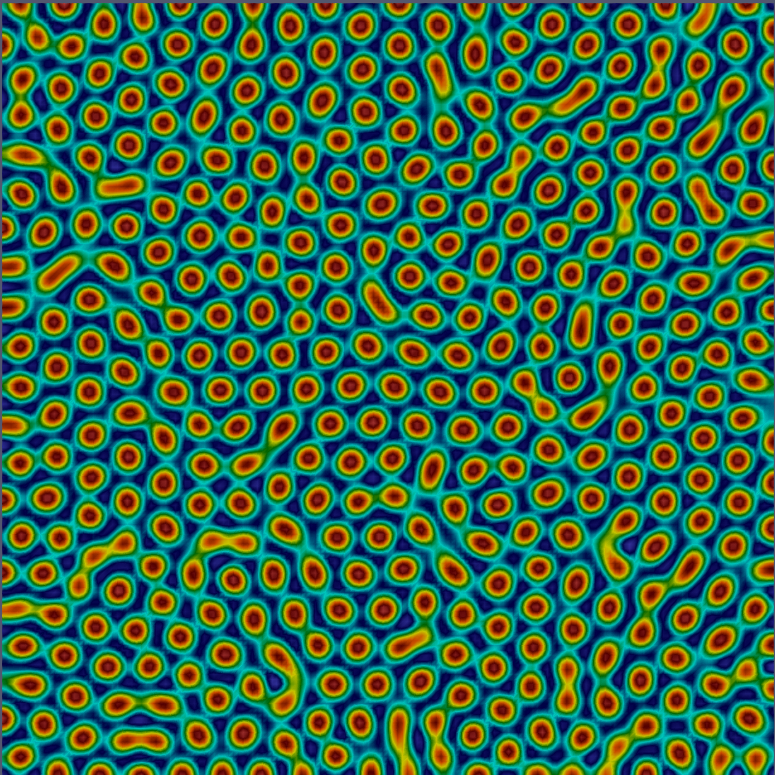
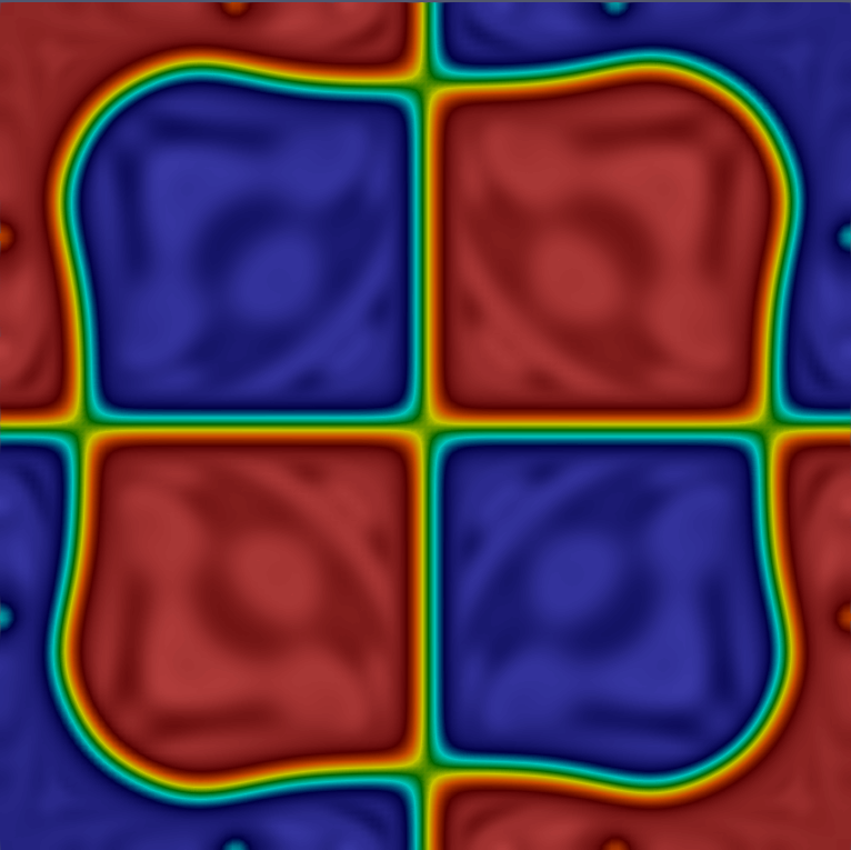
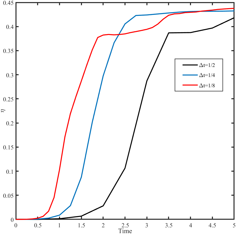
Figure 2: Snapshots of the phase variable $r=0$0 computed by the SAV–CN scheme at $r=0$1. The line graphs give the discrepancy between the auxiliary variable and the original variable.

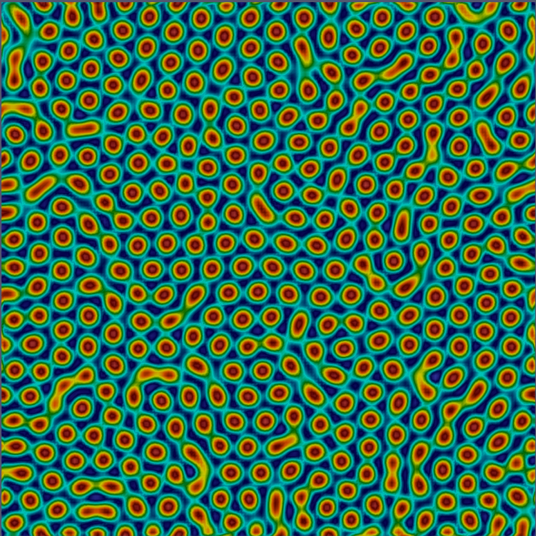
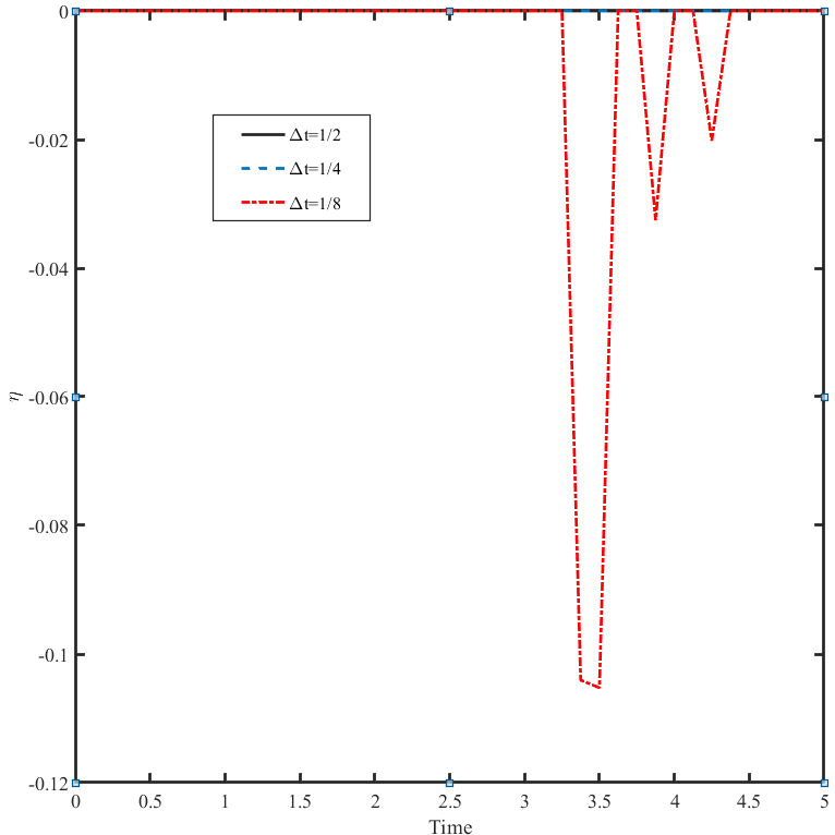
Figure 3: Snapshots of the phase variable $r=0$2 computed by the RAV scheme at $r=0$3. The line graphs give the discrepancy between the auxiliary variable and the original variable.

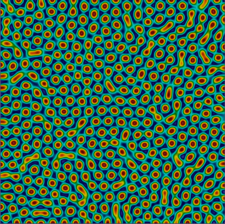
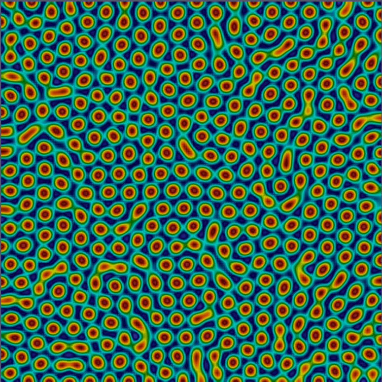
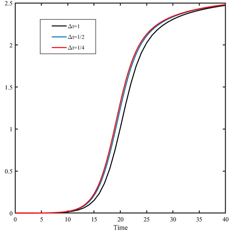
Figure 4: Snapshots of the phase variable $r=0$4 computed by the SAV–CN scheme at $r=0$5. The line graphs give the discrepancy between the auxiliary variable and the original variable.

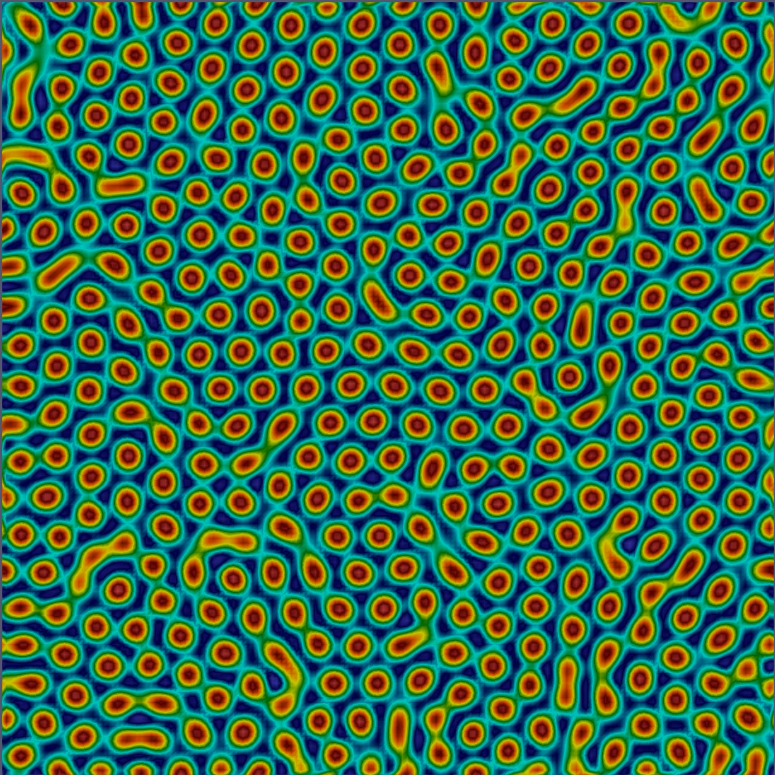
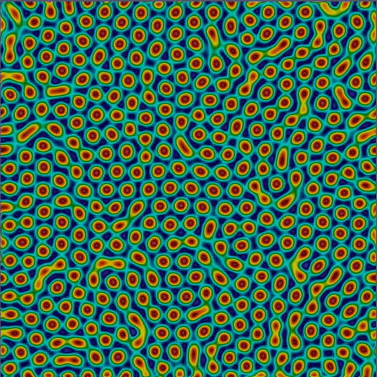
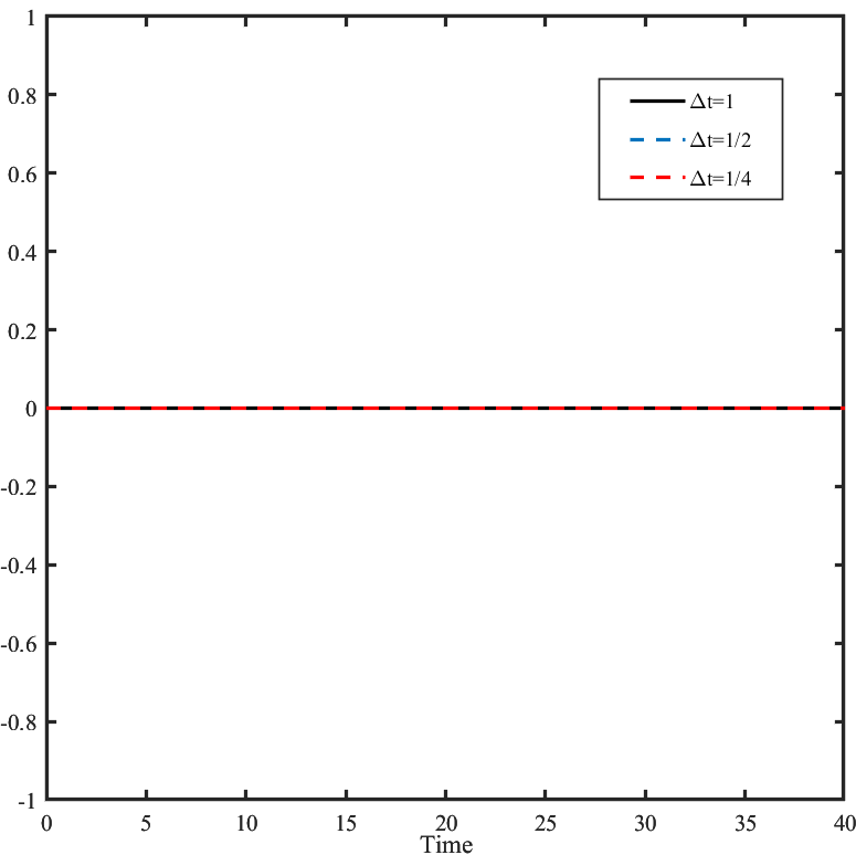
Figure 5: Snapshots of the phase variable $r=0$6 computed by the RAV scheme at $r=0$7. The line graphs give the discrepancy between the auxiliary variable and the original variable.

For high-order accuracy, the paper extends RAV to BDF-$r=0$8 (with explicit coefficients for $r=0$9) and proves corresponding energy laws, though optimal strong-norm error bounds in the high-order setting still require further research.

Practical and Theoretical Implications

• Energy Stability: The RAV approach provides strong dynamical fidelity by ensuring the discrete energy law closely matches the continuum dissipation, free from artificial drift present in other auxiliary variable schemes.
• Step Size Flexibility: The method's error estimates are established with no CFL (step-size) restriction, making the approach suitable for stiff, multiscale problems and large-scale simulations.
• Computational Efficiency: Unlike fully implicit methods, the cost per time step is comparable to IMEX and SAV methods, as the linear systems have constant coefficients and the nonlinearities are handled explicitly.
• Extension to Multi-Field and Multi-Physics Problems: RAV generalizes to gradient flows with multiple fields, e.g., multiphase or coupled surfactant models, enhancing its applicability in complex materials and fluid systems.

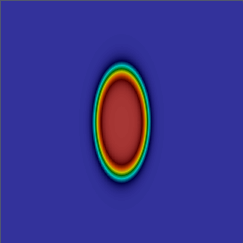
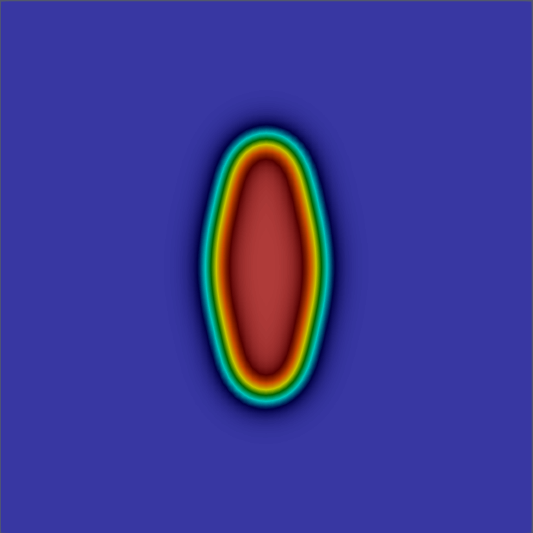
Figure 6: Evolution of a vesicle at different times.

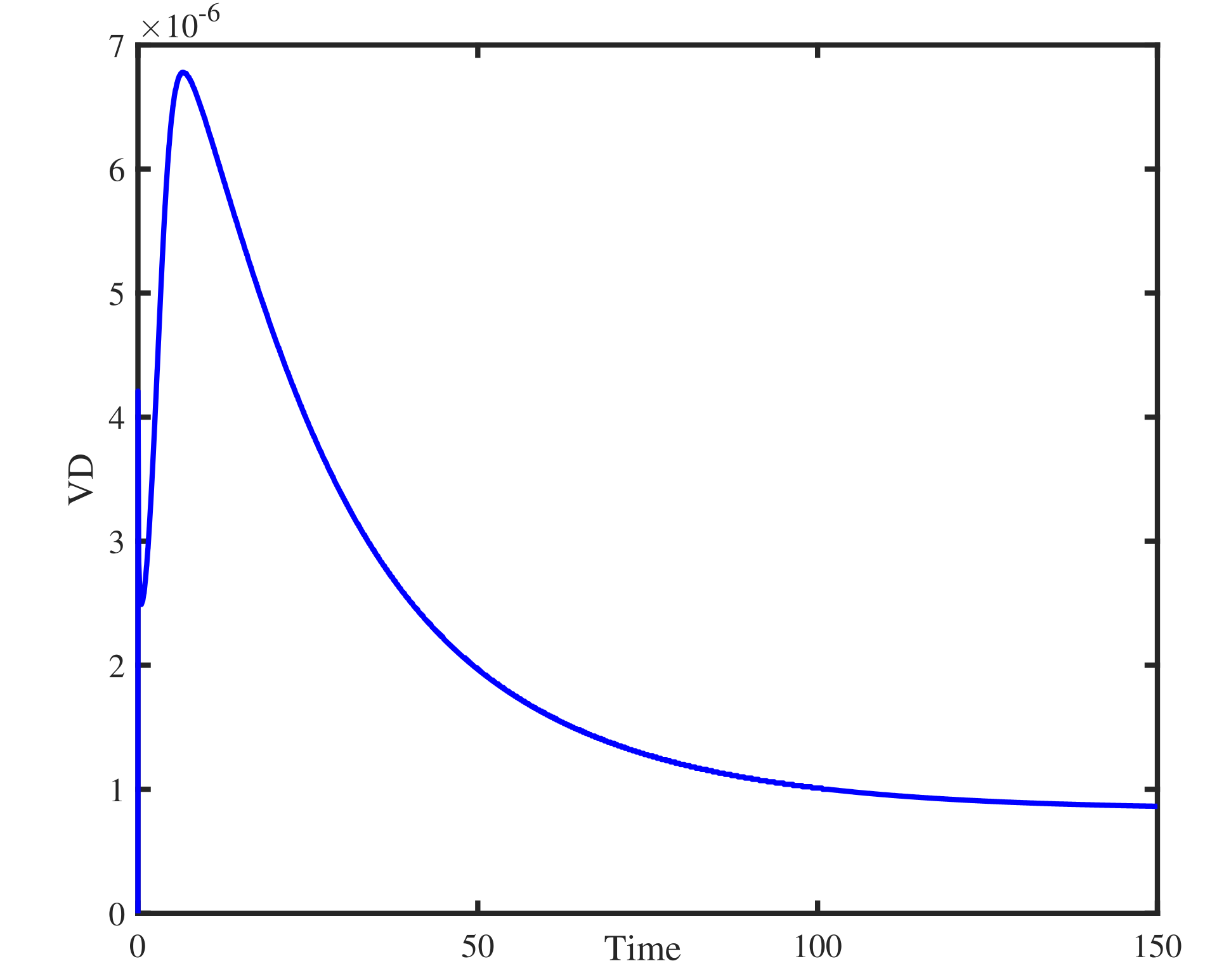
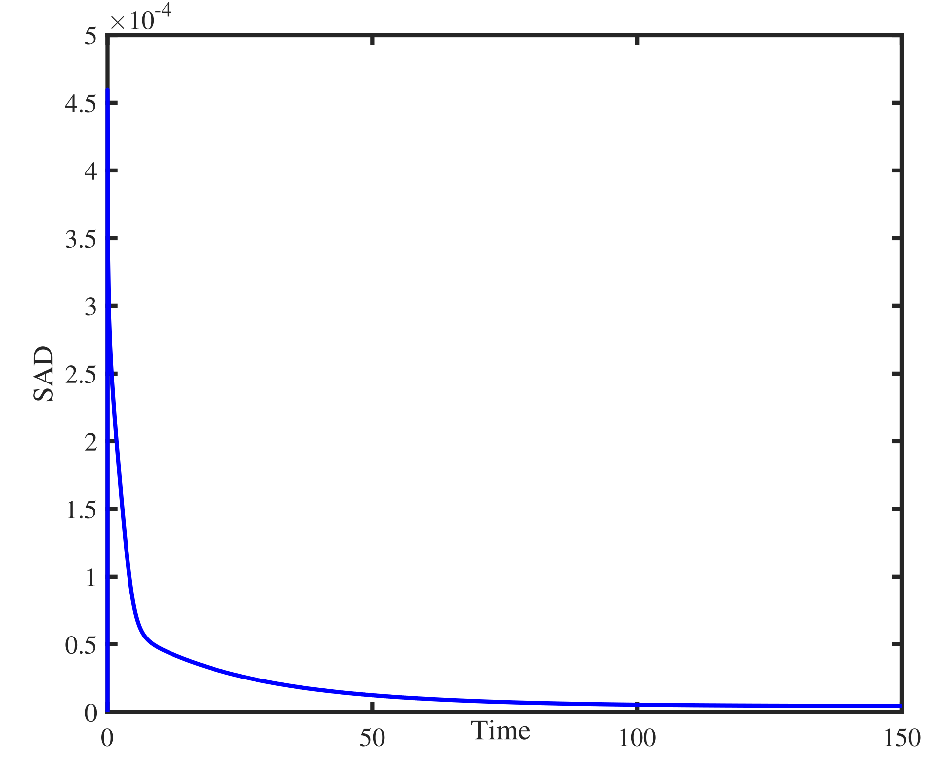
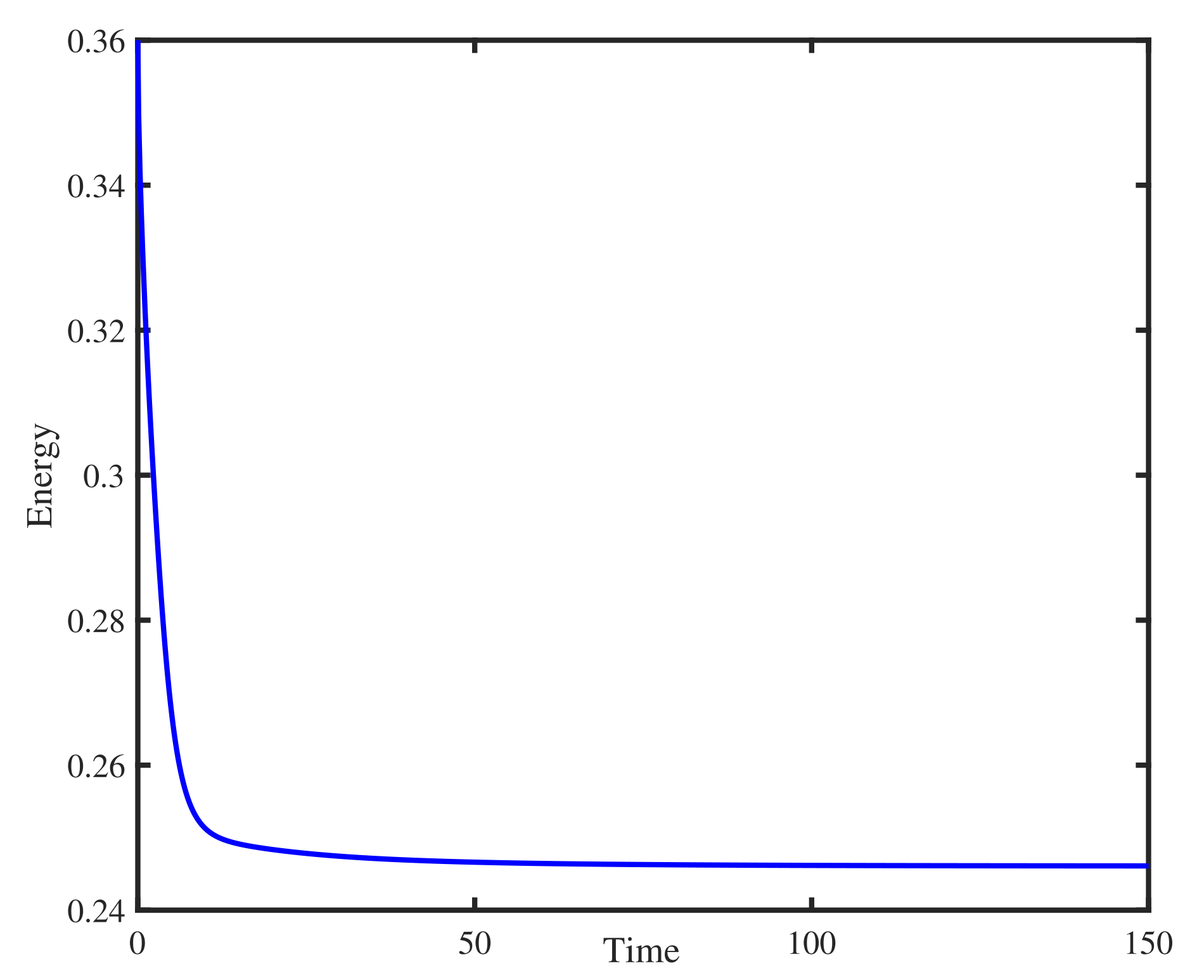
Figure 7: Volume difference, surface area difference, and energy evolution curves.

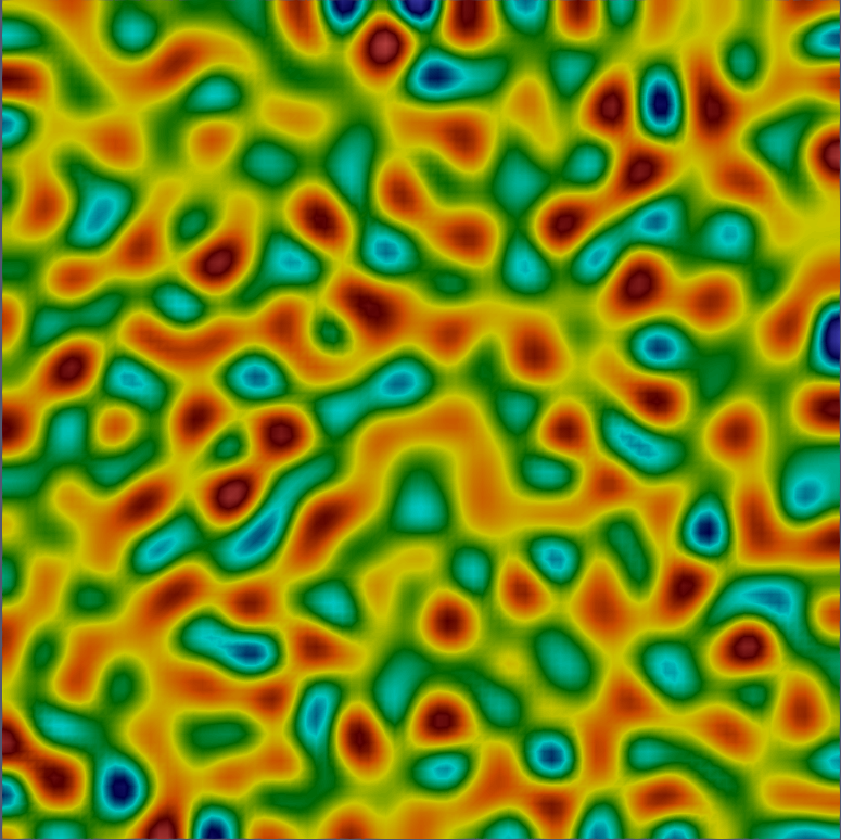
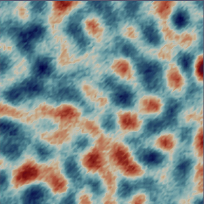
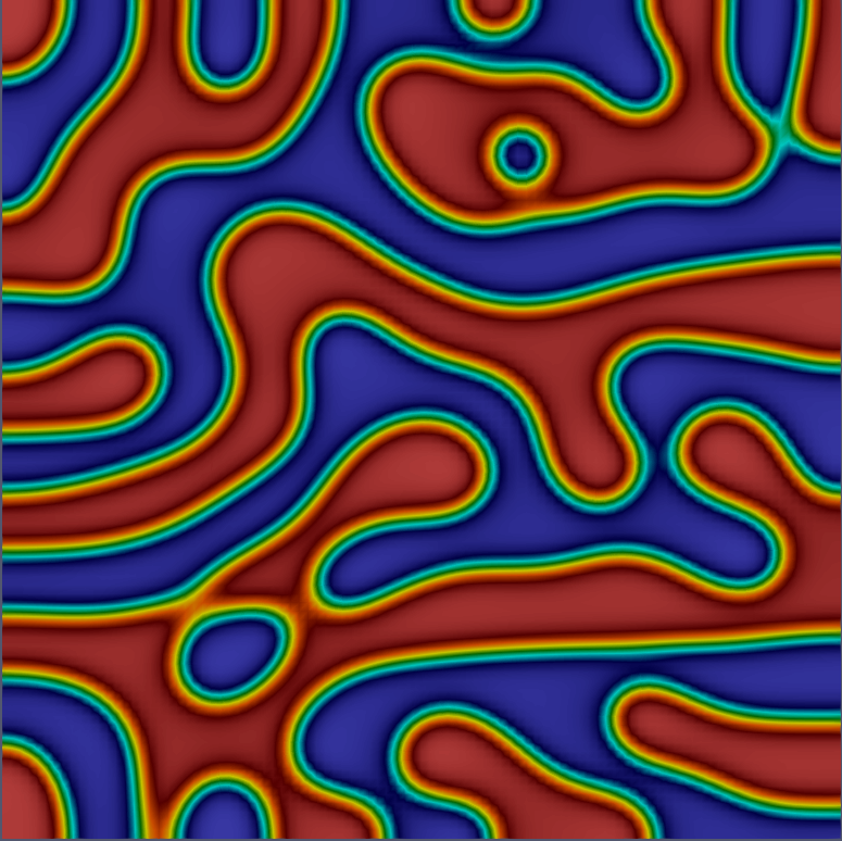
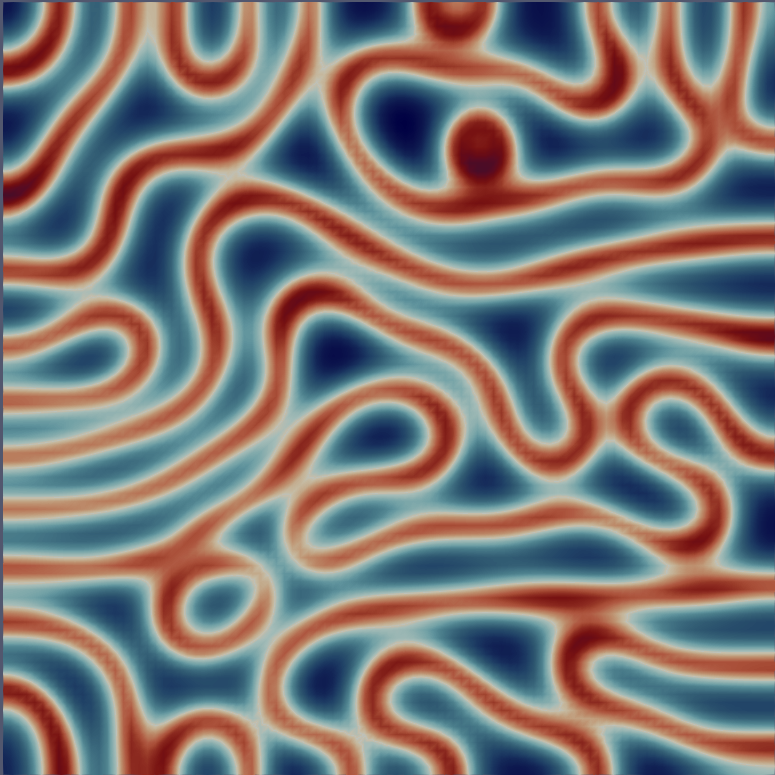
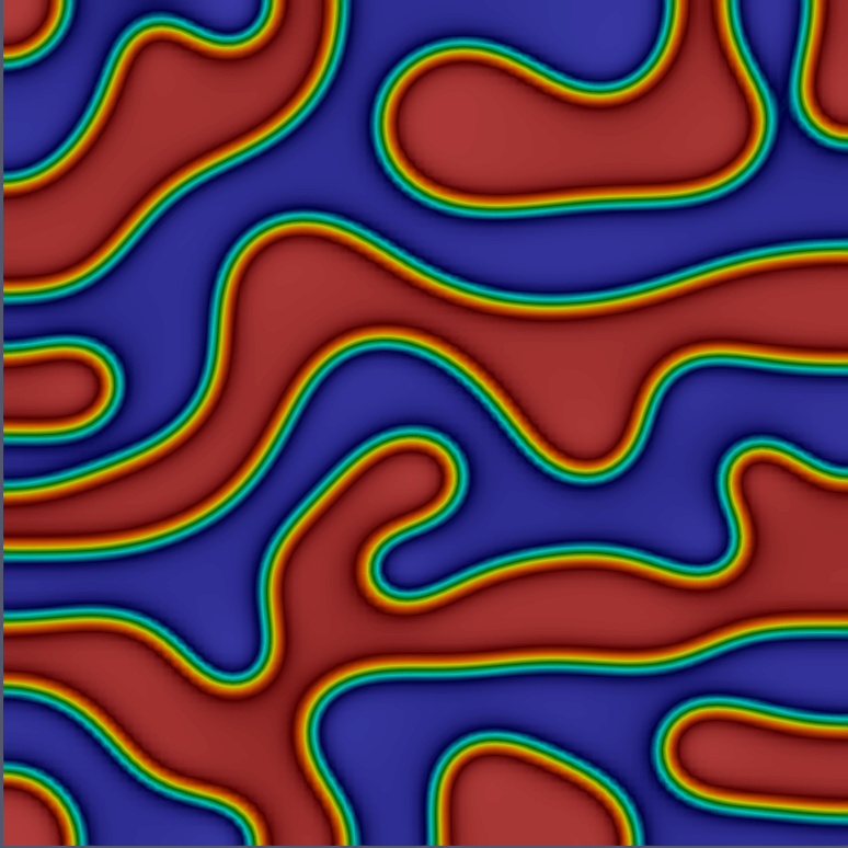
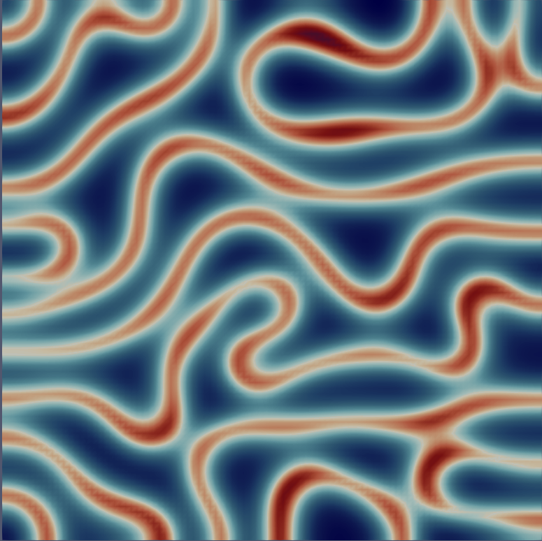
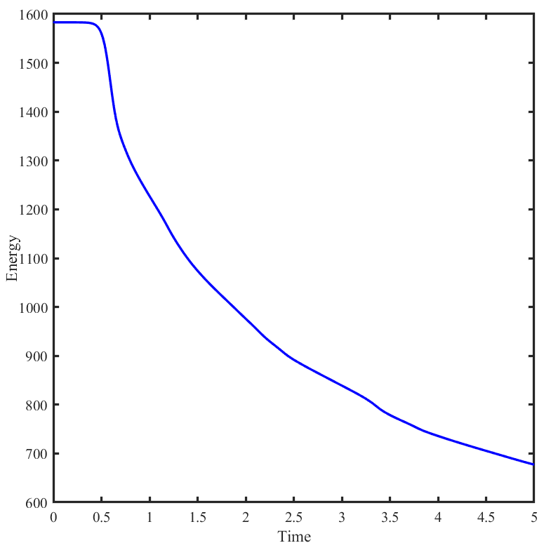
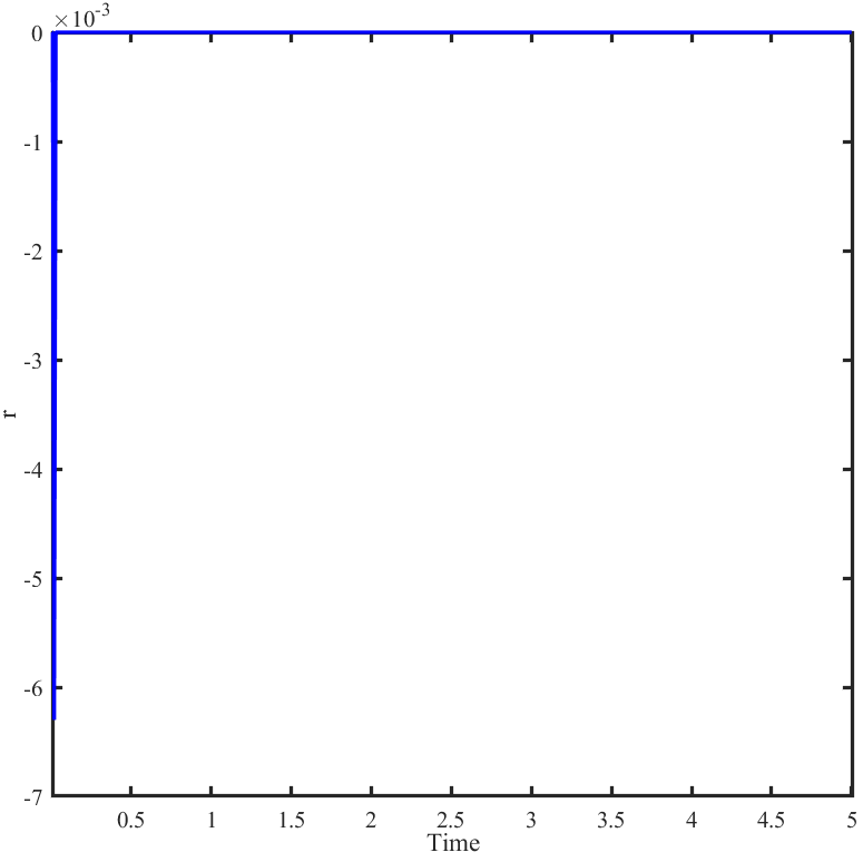
Figure 8: Time evolution of spinodal decomposition and energy dissipation.

Future Directions

The methodology is broadly applicable to dissipative systems beyond gradient flows. Potential future developments include:

• Extension to generalized Navier-Stokes systems and kinetic equations, guided by the analytic and numerical stability provided by the regularized auxiliary structure.
• Development of high-order accurate error analysis for RAV/BDF-$r$0 schemes without step-size restriction.
• Investigation of adaptive and error-controlled strategies leveraging the analytic stability of the RAV framework.

Conclusion

The RAV methodology systematically addresses the consistency and stability limitations of prior auxiliary variable techniques for gradient flow discretization. The approach achieves strict energy stability, strong error control, and computational efficiency. This makes it a robust candidate for the numerical integration of a wide range of nonlinear dissipative PDEs, particularly where accurate long-time dynamics are essential. Theoretical and empirical analysis affirms the RAV approach as a rigorous and practical framework for future research in numerical analysis of gradient flows and related systems (2604.03597).