Microergodicity implies orthogonality of Matérn fields on bounded domains in $\mathbb{R}^4$
Abstract: Matérn random fields are one of the most widely used classes of models in spatial statistics. The fixed-domain identifiability of covariance parameters for stationary Matérn Gaussian random fields exhibits a dimension-dependent phase transition. For known smoothness $ν$, Zhang \cite{Zhang2004} showed that when $d\le3$, two Matérn models with the same microergodic parameter $m=σ2α{2ν}$ induce equivalent Gaussian measures on bounded domains, while Anderes \cite{Anderes2010} proved that when $d>4$, the corresponding measures are mutually singular whenever the parameters differ. The critical case $d=4$ for stationary Matérn models has remained open. We resolve this case. Let $d=4$ and consider two stationary Matérn models on $\mathbb R4$ with parameters $(σ_1,α_1)$ and $(σ_2,α_2)$ satisfying [ σ_12α_1{2ν}=σ_22α_2{2ν}, \qquad α_1\neq α_2. ] We prove that the corresponding Gaussian measures on any bounded observation domain are mutually singular on every countable dense observation set, and on the associated path space of continuous functions. Our approach can be viewed as a spectral analogue of the higher-order increment method of Anderes \cite{Anderes2010}. Whereas Anderes isolates the second irregular covariance coefficient through renormalized quadratic variations in physical space, we detect the first nonvanishing high-frequency spectral mismatch via localized Fourier coefficients and use a normalized Whittle score to identify parameters. More broadly, the localized spectral probing framework used here for detecting subtle covariance differences in Gaussian random fields may be useful for studying identifiability and estimation in other spatial models.
Paper Prompts
Sign up for free to create and run prompts on this paper using GPT-5.
Top Community Prompts
Explain it Like I'm 14
What this paper is about
This paper studies a popular way to model how things vary across space, called a Matérn Gaussian random field. Think of it as a smooth “random landscape” used in spatial statistics. The authors answer a long‑standing question about dimension 4 (four spatial directions): if you observe this random field very densely inside a fixed box, can you tell apart two different Matérn models that look almost the same at small scales?
Their main result: in 4 dimensions, yes—you can tell them apart. More precisely, even if two models share the same “microergodic” combination of parameters (which makes them look nearly identical at very high frequencies), they are still different enough that you can separate them from dense data on any bounded region. This settles the previously open “critical” case of dimension 4.
The big picture and purpose
Matérn models have three key knobs:
- σ² (sigma squared): how big the overall variability is (how tall the bumps are),
- α (alpha): how quickly the field changes across space (the “range” of correlation),
- ν (nu): how smooth the field is (how bumpy vs. silky the surface is).
In many applications, you observe data in a fixed area (like a map region) but at more and more points. This is called fixed‑domain (or “infill”) asymptotics. A core question is: which parameters can you actually learn from a single, very dense set of measurements in that fixed area?
Past results showed a “phase transition” that depends on dimension d:
- For d ≤ 3: if ν is known, you can only learn a certain combination of parameters, called the microergodic parameter m = σ² α{2ν}. You can’t separate σ² and α from each other using one dense sample.
- For d > 4: you can separate σ² and α.
- For d = 4: it was unknown. This paper resolves it.
The main questions in simple terms
- If two Matérn models have the same smoothness ν and the same microergodic parameter m = σ² α{2ν}, but different α (range), can we still tell them apart from dense observations in a fixed 4D region?
- Does dimension 4 behave like “low” dimensions (2–3) where only m is learnable, or like “higher” dimensions (>4) where σ² and α can be separated?
How the authors approach the problem (everyday explanation)
The authors look at the field through the lens of frequency—like analyzing a song by its bass, mid, and treble. High frequencies correspond to very small‑scale wiggles in the field. Two models with the same m have almost the same very high‑frequency behavior to first order, which is why they’re hard to tell apart.
Here’s the key idea:
- They build “localized Fourier coefficients.” This is like focusing your listening to a small patch and measuring how much energy there is at different frequencies, but only using data from inside the observation box (so it’s localized).
- Although the two models have the same leading behavior at high frequencies, the first tiny difference shows up in the next order of the spectrum (think: a very slight difference in treble). For each high‑frequency note, the difference is small—about proportional to 1/(frequency)².
- In 4 dimensions, when you add up these tiny differences across many high‑frequency notes, the total difference grows slowly—only like a logarithm (log N)—but it still grows without bound. This slow growth is just enough to make the two models distinguishable if you gather enough high‑frequency information.
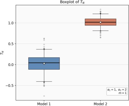
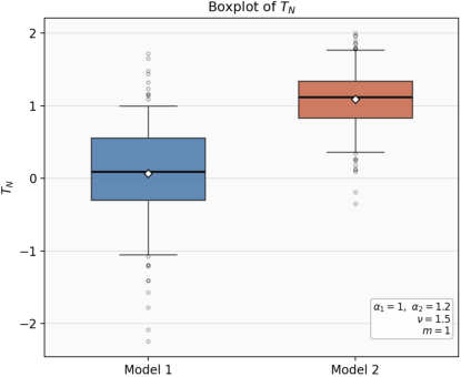
They turn this into a concrete test statistic, called T_N, which:
- averages these small frequency‑wise differences (properly weighted), and
- normalizes by the total “information” across frequencies.
Under one model, T_N tends to 0; under the other, it tends to 1. That means the models are truly different in a way that shows up from dense data in a bounded region.
Why localization matters: the field is only observed inside a bounded box, so straightforward Fourier methods mix frequencies. By multiplying by a smooth “window” function that lives inside the box, the authors carefully control how much different frequencies interfere, making the method work reliably.
What the authors found and why it matters
Main finding:
- In 4 dimensions (d = 4), if two Matérn models have the same ν and the same microergodic parameter m = σ² α{2ν}, but different α, then the probability laws they generate (what a random path looks like) are mutually singular on any bounded observation domain. In simple terms: even if they match at first glance, they are different enough that you can tell them apart with dense data from a fixed region.
Why this is important:
- It closes the gap between known results: for d ≤ 3, you cannot separate σ² and α (only m is learnable); for d > 4, you can separate them; and now for d = 4, you can also separate them.
- Practically, it says that in 4D settings, the “range” α is identifiable from dense data in a fixed area when ν is known, even if two models share the same microergodic combination.
- Conceptually, it explains why dimension 4 is “critical”: the small differences at high frequencies add up just slowly enough (logarithmically) to still make a decisive difference.
They also show:
- Their spectral/localized approach recovers known higher‑dimension results (d > 4) and tightly mirrors earlier physical‑space methods (like using repeated increments) developed by others, notably Anderes (2010).
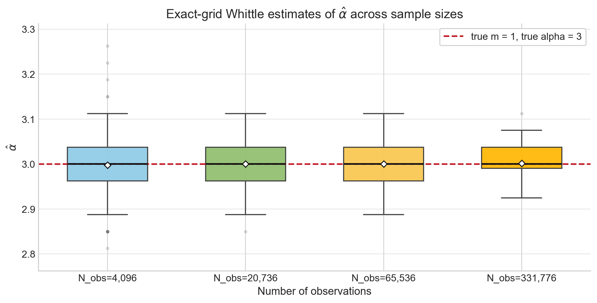
- Their technique connects naturally to “Whittle‑type” frequency‑domain methods and suggests new ways to estimate parameters by pooling many tiny high‑frequency clues.
The paper also includes a small simulation study that illustrates: even when two models have the same m but different α, the test statistic T_N separates them (clustered near 0 for one model and near 1 for the other).
What this means going forward
- For theory: It settles the last open Euclidean case for Matérn fields in fixed domains, pinpointing dimension 4 as the borderline where tiny spectral differences accumulate just enough to matter.
- For practice: In 4D applications (for example, tasks involving three spatial coordinates plus one extra spatial‑like dimension), this supports the use of high‑frequency, localized spectral tools to estimate the range parameter α from dense data.
- For methods: The “localized spectral probing” idea—carefully zooming into high frequencies within a bounded region—could help study identifiability and build new estimators in other spatial models, especially when differences are subtle and spread across many frequencies.
In short: even though two Matérn models can look nearly identical at very small scales if they share m, in four dimensions their tiny differences add up across frequencies. With the right tools, those differences are strong enough to reliably tell the models apart.
Knowledge Gaps
Knowledge gaps, limitations, and open questions
Below is a concise list of what remains missing, uncertain, or unexplored, with concrete directions for future research.
- Unknown smoothness ν: Extend the equivalence/orthogonality and identifiability results to the case where ν is unknown (and possibly jointly estimated), including a full classification of when two Matérn models on bounded domains in d=4 are equivalent or singular when ν differs.
- Complete equivalence classification in d=4: Provide necessary and sufficient conditions for equivalence/orthogonality for all parameter differences (ν, α, σ), not just the microergodic-matched, α1 ≠ α2 case; formally include cases with m1 ≠ m2 and/or ν1 ≠ ν2.
- Estimation theory at the critical information scale: Develop consistent estimators for (α, σ2) in d=4 (e.g., localized Whittle or MLE), establish convergence rates (expected to be at the L_N ~ log N scale), and prove asymptotic normality and efficiency; characterize the optimal rate in local alternatives Δ(α2) = O(1/√log N).
- LAN/contiguity framework: Establish local asymptotic normality in the α2 direction with information L_N ~ log N, derive the Fisher information and optimal tests, and delineate the contiguity region explicitly.
- From subsequence to full-sequence convergence: Replace the sparse subsequence {N_s} required for almost sure separation with either (i) a weighting scheme or block construction that ensures decorrelation, or (ii) a central limit theorem for the score S_N that yields full-sequence convergence and confidence intervals.
- Discrete and irregular sampling: Bridge the continuous-statistic theory to practical observation schemes (grids and irregular designs); quantify Riemann-sum and boundary discretization errors in computing X_k from data; specify sampling densities relative to the maximal frequency N needed for consistency.
- Observation noise (nugget): Incorporate measurement error into the theory; determine how noise alters equivalence/orthogonality in d=4 and how to modify T_N or localized Whittle methods to remain consistent.
- Anisotropy and nonstationarity: Extend the orthogonality result and spectral probing method to anisotropic Matérn models (geometric anisotropy with matrix A) and to nonstationary settings; identify the microergodic combinations and second-order spectral mismatches that remain identifiable in d=4.
- Domain geometry and boundary effects: Quantify how the domain shape and regularity of ∂D affect off-diagonal decay and constants; provide guidance or guarantees for non-smooth or highly irregular domains and for cutoffs χ that touch or approach the boundary.
- Choice and optimization of localization χ and frequency shells: Analyze the impact of χ on information accumulation and variance; design χ and shell-selection rules that maximize L_N and minimize off-diagonal leakage; provide data-driven tuning procedures.
- Robustness to model misspecification: Study whether the score-type approach remains consistent when the true covariance is only Matérn-like at high frequencies (e.g., correct tail exponent but incorrect low-frequency behavior); develop semiparametric conditions under which α remains identifiable at the log scale.
- Relationship to tapering and pseudo-likelihood: Provide theory for the consistency, rates, and efficiency of taper-based and localized-Whittle estimators for α in d=4; determine when tapering preserves the O(log N) information and how to optimally select tapers.
- Trend and mean uncertainty: Extend results to unknown mean or low-frequency trend components; develop procedures that remove or project out trends without sacrificing the subtle high-frequency signal needed for identifiability in d=4.
- Multivariate and cross-covariance Matérn: Generalize to multivariate Matérn fields; characterize which combinations of cross-range parameters are microergodic in d=4 and whether second-order spectral mismatches yield orthogonality.
- Beyond Euclidean domains: Formalize analogues on compact manifolds or periodic domains by replacing Fourier modes with eigenfunctions; characterize the criticality analogous to d=4 via Weyl’s law on general geometries and boundary conditions.
- Minimal-design conditions: Identify minimal sampling conditions (e.g., density on a subset of D, or along submanifolds) that still allow separation at the O(log N) information scale; determine failure modes when the design is insufficiently dense or spatially non-uniform.
- Finite-sample testing and power: Turn the separation statistic T_N into finite-sample hypothesis tests with size and power guarantees; calibrate critical values under dependence and off-diagonal leakage; quantify power against local alternatives Δ(α2) = c/√log N.
- Numerical and computational aspects: Provide implementable algorithms (and code) for computing T_N from spatial-domain data (not just spectral simulations), including FFT-based approximations, complexity analysis, and guidance on choosing K0, N, and χ for finite samples.
- Interaction with operator-based bounded-domain models: Extend the comparison with Whittle–Matérn operator models to variable-coefficient operators and boundary conditions; clarify when the stationary-restriction and intrinsic-operator formulations yield the same equivalence thresholds in d=4.
Practical Applications
Overview
This paper resolves a long‑standing open question in spatial statistics: for stationary Matérn Gaussian random fields on bounded domains in four dimensions (d = 4) with known smoothness ν, the variance (σ²) and range (α) parameters are separately identifiable under fixed‑domain (infill) asymptotics, even when the microergodic combination m = σ²α{2ν} matches. Concretely, the authors prove that two Matérn models with the same m but different α induce mutually singular Gaussian measures on any bounded domain in ℝ⁴, which implies that α is asymptotically estimable in d ≥ 4 (and in d = 4 at a slow, logarithmic information rate). They introduce a practical “localized spectral probing” framework based on localized Fourier coefficients and a normalized Whittle‑type score statistic that aggregates weak high‑frequency discrepancies to separate models.
Below are practical applications that derive from these findings and methods, organized by deployment horizon and mapped to sectors, tools, workflows, and key assumptions.
Immediate Applications
The following applications can be prototyped or deployed now using existing statistical and computing tooling (e.g., FFTs, tapering, GP libraries, INLA/SPDE, Python/R).
- Parameter estimation and hypothesis testing for 4D Matérn fields using localized spectral probes
- What to do: Implement the paper’s localized Fourier coefficient workflow with a smooth, compactly supported window χ and compute the normalized score statistic T_N (or a localized Whittle pseudo‑likelihood) to estimate or test α when ν is known.
- Sectors:
- Healthcare/Neuroscience: 3D+time imaging (e.g., 4D fMRI, dynamic CT) model‑based denoising and interpolation.
- Energy/Geoscience: 4D seismic (3D subsurface + time) monitoring for reservoir characterization.
- Climate/Earth sciences: 3D reanalysis cubes over short time windows modeled as quasi‑stationary 4D fields.
- Software/ML: Gaussian process (GP) hyperparameter estimation in 4D inputs.
- Tools/workflows:
- Compute localized Fourier coefficients X_k via FFTs with taper χ; estimate smoothed variances v_j(k) = (f_j ∗ |χ̂|²)(k); form score or Whittle objective and optimize α.
- Integrate as a module in Python (NumPy/SciPy/pyFFTW), R (fft, Matrix, fields), or GP libraries (GPyTorch, scikit‑gp).
- Assumptions/dependencies:
- Known smoothness parameter ν.
- Approximate stationarity and (near‑)isotropy in the 4D domain.
- Dense sampling on a bounded domain; variance information accumulates only logarithmically in d=4, so adequate high‑frequency coverage is needed.
- Observation noise should be modeled or pre‑whitened in the pseudo‑likelihood.
- Model validation and diagnostic for range parameter misspecification
- What to do: Use T_N as a goodness‑of‑fit diagnostic to detect whether a candidate α matches the data (under fixed m), or to compare two fitted 4D Matérn models.
- Sectors: All Matérn‑using domains above.
- Tools/workflows:
- Fit m (or m and ν) via conventional methods; fix m, sweep candidate α values and use T_N to flag misfit.
- Assumptions/dependencies:
- Same as above; diagnostic power improves with denser sampling and broader frequency reach.
- Sampling design guidance for 4D fields
- What to do: When collecting dense 4D data in bounded domains, ensure enough resolution to capture high‑frequency content so that α is identifiable; be aware that in ≤3 dimensions this separation is not feasible asymptotically for known ν.
- Sectors: Environmental monitoring networks (3D arrays + time), industrial sensing, medical imaging protocols.
- Tools/workflows:
- Pre‑study simulations with the paper’s frequency‑space simulator to quantify how large shells (N) must be to achieve desired precision on α.
- Assumptions/dependencies:
- Trade‑off between acquisition cost and the slow log‑scale information growth in d=4.
- Improved Bayesian priors and model specifications in 4D INLA/SPDE pipelines
- What to do: In SPDE/INLA workflows for Matérn‑type fields in 4D, treat the range (κ or α) as separately identifiable (given ν,m), and avoid overly informative priors that tie κ to τ when ν is fixed.
- Sectors: Geostatistics, environmental epidemiology, spatio‑temporal risk mapping.
- Tools/workflows:
- Adjust priors in INLA/Template Model Builder; include localized spectral score diagnostics in posterior predictive checks.
- Assumptions/dependencies:
- Appropriate mesh resolution and boundary conditions on bounded domains; near‑stationarity within analysis windows.
- Teaching and reproducible demos for identifiability in spatial stats
- What to do: Use the paper’s simulation code structure to demonstrate the d=4 criticality and log‑scale accumulation of information in advanced spatial statistics courses.
- Sectors: Academia/education.
- Tools/workflows:
- Classroom notebooks implementing localized spectral probing and comparing d=3 vs d=4 behavior.
- Assumptions/dependencies:
- Students can run FFT‑based simulations; ν is fixed in examples.
Long‑Term Applications
The following targets require further research, engineering, or generalization beyond the current paper (e.g., handling nonstationarity, unknown ν, irregular sampling, or large‑scale deployment).
- End‑to‑end localized Whittle estimators and tests for 4D Matérn models at scale
- What to build: Robust estimators and test suites that combine localized spectral probing with automatic window design (χ), shell selection, noise modeling, and uncertainty quantification for α and σ², with options to estimate ν.
- Sectors: Software/ML, geoscience platforms, medical imaging suites.
- Tools/products:
- Open‑source packages (Python/R) with GPU‑accelerated localized FFTs and batched shells; integration with GPyTorch/Stan/INLA.
- Assumptions/dependencies:
- Efficient handling of off‑diagonal terms introduced by localization; scalable memory and compute.
- Extension to non‑isotropic and non‑stationary 4D spatio‑temporal models
- What to research: Adapt the localized spectral framework to anisotropic or nonseparable spatio‑temporal Matérn variants, and to locally stationary models where stationarity holds only within windows.
- Sectors: Climate and weather nowcasting, 4D MRI/fNIRS, industrial process monitoring.
- Tools/workflows:
- Multi‑window (spatial/temporal) χ with adaptive bandwidths; composite likelihood across patches; anisotropic score weights using directional derivatives.
- Assumptions/dependencies:
- Careful bias‑variance trade‑offs due to windowing; validated asymptotic theory beyond strict stationarity/isotropy.
- Irregular designs and measurement noise
- What to research: Generalize localized Fourier probing to irregular grids and noisy observations (e.g., by constructing approximate localized spectral transforms or using reproducing kernel Hilbert space projections).
- Sectors: Remote sensing, sensor networks, mobile robotics.
- Tools/workflows:
- Non‑uniform FFTs (NUFFTs) or graph‑spectral surrogates; deconvolution/noise‑aware pseudo‑likelihoods.
- Assumptions/dependencies:
- Stable NUFFT implementations; identifiability may degrade with strong noise or sparse high‑frequency coverage.
- Optimal window (taper) and shell design for maximal information gain
- What to research: Design χ and shell strategies that maximize L_N (the information scale) subject to numerical stability and edge effects, and quantify finite‑sample efficiency.
- Sectors: All applied sectors using Matérn models.
- Tools/workflows:
- Optimization over taper families (e.g., prolate spheroidal tapers), adaptive shell widths, cross‑validation of bias/variance.
- Assumptions/dependencies:
- Domain geometry and boundary effects influence χ̂ decay and off‑diagonal covariance.
- Spatio‑temporal mapping and SLAM with learned correlation ranges
- What to build: Online estimators for α within 3D‑space‑plus‑time GP models for mapping and tracking, leveraging localized spectral statistics over sliding 4D windows.
- Sectors: Robotics/autonomous systems, AR/VR, 4D mapping.
- Tools/workflows:
- Streaming localized FFTs, incremental score updates, embedded GPU deployment.
- Assumptions/dependencies:
- Approximate local stationarity in short time windows; known or profiled ν; real‑time computational budgets.
- Domain‑specific 4D pipelines
- Energy/Geoscience (4D seismic): Incorporate α‑aware inference in history matching and reservoir monitoring to reduce bias from conflating m with α; integrate with adjoint/PDE workflows.
- Healthcare (4D imaging): Improve variance/range separation in dynamic reconstructions and uncertainty quantification for image‑guided interventions.
- Climate/Earth system reanalysis: Use localized spectral probes to calibrate correlation ranges in 4D assimilation windows for better downscaling and forecasting.
- Tools/workflows:
- Coupled GP‑PDE or GP‑data assimilation pipelines; modular α‑estimation callable as a service.
- Assumptions/dependencies:
- Windowed stationarity; adequate resolution to access high‑frequency shells; careful treatment of boundaries and noise.
- Policy and standards for 4D data collection and reporting
- What to craft: Guidelines that in 4D settings, α is asymptotically identifiable (given ν), whereas in ≤3D it is not—impacting how agencies design sampling campaigns and report uncertainty.
- Sectors: Environmental regulation, public health surveillance, national statistics.
- Tools/workflows:
- Pre‑deployment power analyses using the paper’s framework to justify sensor density and resolution; standardized reporting of (m, α, ν).
- Assumptions/dependencies:
- Cross‑stakeholder agreement on modeling assumptions (Matérn class, stationarity within campaign windows).
Cross‑cutting assumptions and dependencies (affecting feasibility)
- Known smoothness ν: The main identification results and proposed statistic T_N assume ν is given; estimating ν reliably may require additional techniques and stronger data.
- Stationarity and isotropy in 4D: Results are derived for stationary, isotropic Matérn fields on bounded domains; departures (e.g., strong anisotropy, nonstationarity, nonseparable time effects) require extensions.
- Dense infill asymptotics: Practical performance depends on sufficiently fine sampling; in d=4, information grows only like log N, so gains can be slow and require high resolution.
- Bounded domain handling: The method leverages compactly supported tapers χ wholly inside the observation domain; edge effects and domain geometry matter.
- Off‑diagonal covariance control: Localized spectral coefficients are only approximately diagonal; robust software must control induced correlations for valid inference.
- Observation noise and model mismatch: Noise and deviations from the Matérn family need to be accounted for in pseudo‑likelihoods and diagnostics to avoid biased conclusions.
These applications turn the paper’s theoretical resolution of the d=4 critical case and its localized spectral probing method into tangible workflows for parameter estimation, model checking, and sampling design in 4D datasets across science and industry.
Glossary
- Bochner's theorem: A result that characterizes positive-definite functions as Fourier transforms of finite measures; it yields the spectral representation of stationary covariances. "By Bochner's theorem, "
- Cameron--Martin condition: A condition describing when Gaussian measures with different means are equivalent, requiring the mean difference to lie in a certain Hilbert space. "together with the corresponding Cameron--Martin condition on the means."
- circular complex Gaussian: A complex Gaussian variable that is rotationally invariant in the complex plane (real and imaginary parts i.i.d. with equal variance and zero pseudo-mean). "independent, centered, circular complex Gaussian with"
- Dirichlet boundary conditions: Boundary conditions fixing a function to be zero on the boundary of a domain. "with homogeneous Dirichlet boundary conditions."
- Dirichlet Laplacian: The Laplace operator on a domain equipped with Dirichlet boundary conditions (vanishing on the boundary). "the th eigenvalue of the Dirichlet Laplacian on "
- Fourier transform: An integral transform to frequency space; used here to express covariances and define spectral densities. "We use the Fourier transform convention"
- Gaussian measures: Probability measures induced by Gaussian processes on function or sequence spaces; their equivalence or singularity affects estimability. "induce equivalent Gaussian measures on bounded domains,"
- Gaussian random fields: Collections of random variables indexed by space where every finite set is jointly Gaussian. "Gaussian random fields are a central tool for modeling spatial dependence"
- high-frequency tail: The asymptotic decay behavior of the spectral density for large frequencies, which drives local regularity and estimability. "This high-frequency tail is fundamental for fixed-domain asymptotics."
- identifiability: The property that different parameter values imply distinguishable distributions; crucial for consistent estimation. "asks which covariance parameters are identifiable, and therefore estimable"
- infill asymptotics: Asymptotic regime where the observation domain is fixed and sampling becomes dense. "This is the fixed-domain, or infill, asymptotic regime."
- isotropy: The assumption that covariance depends only on distance, not direction. "assume isotropy, meaning that there exists a function"
- Kolmogorov's continuity theorem: A theorem guaranteeing a continuous modification of a stochastic process given suitable moment bounds. "Kolmogorov's continuity theorem yields a continuous modification"
- localized Fourier coefficients: Integrals of the field against localized oscillatory functions to probe frequency content in space. "we ``probe'' the field by constructing localized Fourier coefficients."
- Matérn: A widely used parametric class of covariance functions (and corresponding random fields) controlled by variance, range, and smoothness parameters. "Mat " ern random fields are one of the most widely used classes of models in spatial statistics."
- microergodic parameter: The combination m = σ²α{2ν} that determines leading spectral scale and equivalence classes under infill asymptotics. "two Mat " ern models with the same microergodic parameter"
- modified Bessel function of the second kind: Special function Kν appearing in the Matérn covariance formula. "where is the modified Bessel function of the second kind"
- mutually singular: A property of two measures that assign probability one to disjoint sets (orthogonality), implying perfect distinguishability. "the corresponding measures are mutually singular whenever the parameters differ."
- path space: The space of sample paths, here continuous functions on a compact domain, on which Gaussian measures are defined. "on the associated path space of continuous functions."
- pseudo-covariances: Second-order moments of complex random variables of the form E[XX], relevant for noncircular dependencies. "covariances and pseudo-covariances introduced by localization."
- renormalized quadratic variations: Scaled sums of squared increments used to isolate specific coefficients in covariance expansions. "through renormalized quadratic variations in physical space"
- Schwartz function: A smooth function whose derivatives decay faster than any polynomial; used here for the Fourier transform of a smooth compactly supported cutoff. "is a Schwartz function \cite[Theorem 1.13]{duo2024fourier}: for every "
- spectral density: The function f(ξ) giving the power distribution across frequencies; Fourier transform of the covariance. "the spectral density is \cite[p. 49]{stein1999}"
- spectral domain: Frequency space; analyzing covariance models via their spectra rather than directly in physical space. "work in the spectral domain."
- stationary Gaussian field: A Gaussian field with translation-invariant finite-dimensional distributions (covariance depends only on differences). "be a mean-zero stationary Gaussian field"
- tapering: Modifying a covariance (or data) by multiplying with a compactly supported function to localize or regularize estimation. "Classical lag tapering \cite{zhang2008covariance} replaces the stationary covariance kernel by"
- Tonelli--Fubini: Theorems allowing interchange of integration and expectation (or double integrals) under integrability conditions. "we interchange expectation and integration by Tonelli--Fubini,"
- Weyl's law: Asymptotic law for the growth of Laplacian eigenvalues in a domain, linking spectral quantities to dimension and volume. "Since Weyl's law gives "
- Whittle pseudo-likelihood: An approximate likelihood constructed in the frequency domain for Gaussian time series/fields. "based on the Whittle pseudo-likelihood recovers the parameter ."
- Whittle score: The derivative (score) of the Whittle log-likelihood, used here in a normalized form to detect parameter differences. "use a normalized Whittle score to identify parameters."
- Whittle--Mat " ern fields: Gaussian fields defined via fractional elliptic operators (e.g., L{−β}) producing Matérn-type covariances on bounded domains. "generalized Whittle--Mat " ern fields on a bounded domain"
Collections
Sign up for free to add this paper to one or more collections.