Posterior inference via Hill's prediction model
Abstract: This paper is concerned with the construction of prior free posterior distributions which rely on the use of one step ahead predictive distribution functions. These are typically more straightforward to motivate than prior distributions. Recent interest has been with Hill's $A_n$ prediction model through what has become known as conformal prediction. This model predicts the next observation to lie with equal probability in the intervals created by the observed data. The prediction model generates complete data sets which can be used to provide posterior inference on any statistic of interest.
Paper Prompts
Sign up for free to create and run prompts on this paper using GPT-5.
Top Community Prompts
Explain it Like I'm 14
Posterior Inference via Hill’s Prediction Model — Explained Simply
What is this paper about?
This paper shows a new way to measure uncertainty about things we care about (like a mean, variance, or a model parameter) without having to choose a “prior.” Instead of modeling how the data were made, the authors model what we haven’t seen yet: they build a rule for predicting the next data point, then use that to simulate many possible “future” data sets. From these simulated futures, they create a “posterior” (an updated belief) for any quantity of interest.
A key piece is Hill’s prediction model—today often called conformal prediction—where the next data point is assumed to be equally likely to fall into any of the gaps formed by the sorted existing data, and then chosen uniformly within that gap.
1) Main idea in plain terms
Imagine you’ve watched the first half of a sports season and want to guess a team’s final average score. Rather than arguing about a prior belief, this method:
- Focuses on predicting the next game’s score based on what you’ve seen.
- Repeats that “predict the next game” step many times to simulate the rest of the season.
- Uses the simulated full season to compute the final average score many times.
- Treats the spread of those averages as your uncertainty (your “posterior”) about the true final average.
This way, you quantify uncertainty by predicting and simulating the unobserved part, not by assuming a complex model or picking a prior.
2) What questions are they asking?
- Can we build Bayesian-style “posterior” beliefs without picking a prior, just by focusing on how to predict the next data point?
- Does Hill’s simple prediction rule lead to valid, well-behaved uncertainty summaries?
- Can this approach work not only for one variable at a time, but also for several variables together (like pairs or many features) while keeping the same simple, fair prediction idea?
3) How do they do it? (Methods with analogies)
The one-step-ahead prediction approach
- Think of your data as points on a number line, sorted from smallest to largest.
- Hill’s rule says the next point is equally likely to land in any of the “gaps” between these sorted points (including the end gaps), and uniformly within the chosen gap. This is like saying, “I’ll place the next dot somewhere between the existing dots, giving each gap a fair chance.”
Why this is appealing:
- It’s simple, uses only the current data, and doesn’t assume a detailed mathematical model of how the data were generated.
- It creates new values (not just re-using old ones), so it works well for continuous data.
Building a posterior from predictions
- Repeat the “predict the next point” step to simulate many future points until you have a large, “completed” dataset.
- Compute the statistic you care about (like the mean or correlation) on this completed dataset.
- Repeat the whole process many times. The distribution of the results is your “posterior”—your updated belief about the true value.
Why it works (intuition)
- The authors show that, as you keep predicting more points with Hill’s rule, the simulated sequence behaves more and more like draws from some stable underlying distribution (this is called “asymptotic exchangeability,” meaning order doesn’t matter in the long run).
- When this happens, the distribution of your statistic settles down to a stable “posterior.”
Extending to many variables (copulas)
For two or more variables (like height and weight together), they:
- Apply Hill’s rule separately to each variable (so each variable’s next value is predicted fairly across its own gaps).
- Then “glue” the variables together using a copula (specifically a Gaussian copula), which is a mathematical tool that ties together separate variables’ behaviors to control their dependence (like correlation) while keeping each variable’s own behavior intact.
- They update the correlation over time from the simulated data using simple recursive formulas, and show that these correlations settle down (converge) too.
Analogy for a copula:
- Think of baking: marginals are the individual ingredients (flour, sugar), and the copula is the recipe that mixes them to get the final texture (how variables move together).
4) What did they find, and why does it matter?
Main findings:
- Hill’s prediction model leads to sequences of simulated future data that are “asymptotically exchangeable” (loosely, order doesn’t matter in the limit), which supports the existence of a well-defined posterior for any statistic you care about.
- They design new bivariate and multivariate versions that:
- Keep Hill’s simple rule for each variable (fair across gaps).
- Use a Gaussian copula to maintain and update dependence (correlation) across variables.
- Are proven to converge, so they also produce stable posteriors in multiple dimensions.
Illustrations (simulations):
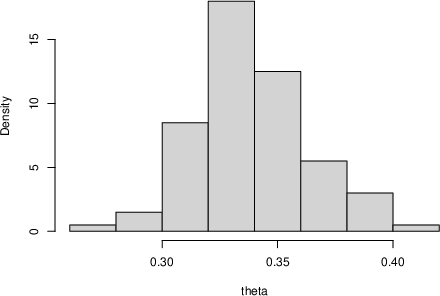
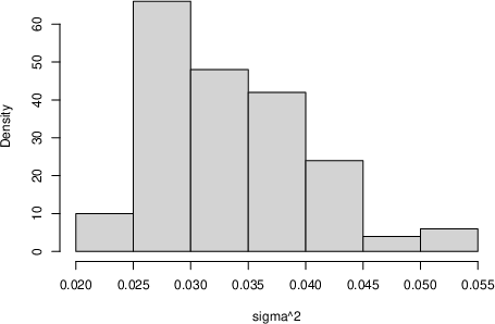
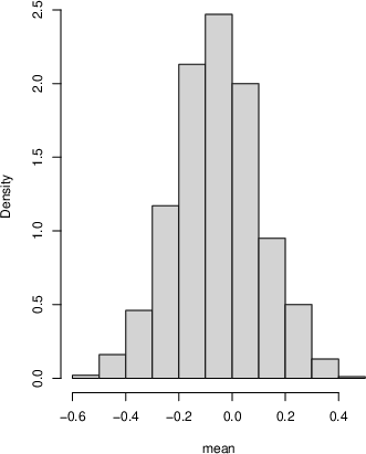
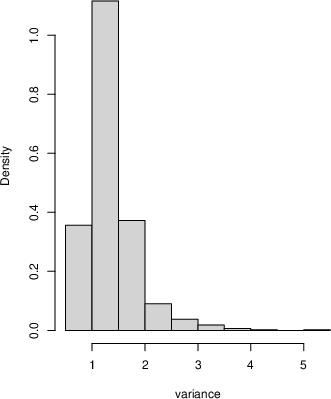
- For simple datasets (like samples from a Beta or Normal distribution), the approach produces sensible posterior distributions for the mean and variance.
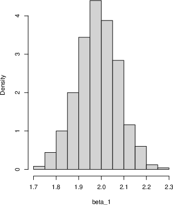
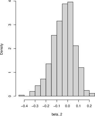
- For linear regression, they simulate future residuals using Hill’s idea (after a transformation to a 0–1 scale and back) and get posterior samples for the regression coefficients that are close to the true values.
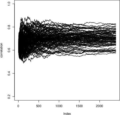
- For two variables, they show trajectories of the estimated correlation converging to different limits across runs—each limit is a sample from the correlation’s posterior.
Why it matters:
- No prior needed: This avoids debates and difficulties about choosing priors, especially in complex models.
- Simple and broadly applicable: Hill’s rule is easy to implement and doesn’t require heavy modeling assumptions.
- Creates new values: Unlike some resampling methods (like the Pólya-urn/Bayesian bootstrap), Hill’s approach can generate new, continuous values rather than only re-using observed ones.
- Connects prediction and inference: It links conformal prediction (a modern, distribution-free prediction tool) to Bayesian-style uncertainty quantification.
5) What could this change?
- Practical uncertainty quantification: You can get posteriors for means, variances, correlations, and regression parameters without picking a prior or fitting complicated likelihood models.
- Multivariate and machine learning settings: The copula-based extension means you can handle multiple features and their relationships, connecting naturally to modern ML tasks where uncertainty matters.
- Transparent assumptions: Because the whole approach is driven by a simple “next-point” rule, it’s easy to explain and audit. Different prediction rules could be plugged in when appropriate.
In short, the paper shows that by focusing on how to predict the next data point (fairly and simply), you can build a full system to measure uncertainty after seeing data—without priors—and extend it to multiple variables in a principled way.
Knowledge Gaps
Knowledge gaps, limitations, and open questions
Below is a focused list of concrete gaps and unresolved questions that the paper leaves open, organized by theme to guide future research.
- Foundational coherence and scope
- Formal coherence of the “posterior” across multiple statistics: the paper asserts that any statistic can be computed from completed datasets, but it does not establish whether joint inference over multiple statistics is coherent (i.e., whether there exists a single joint posterior measure on the data-generating distribution that induces all marginal “posteriors” for functionals consistently).
- Relationship to Bayesian posteriors: beyond conceptual distinctions, the paper does not characterize when (if ever) the proposed posterior coincides with or approximates Bayesian posteriors (e.g., under Bernstein–von Mises type conditions), nor when it diverges and how.
- Frequentist calibration: there is no theoretical analysis of coverage/calibration of credible intervals derived from the proposed posterior, either marginally or uniformly in .
- Asymptotic theory and consistency
- Posterior consistency for general functionals: outside of an illustrative normal-mean example, there is no general theorem establishing that the posterior concentrates at the true value $\theta^\*$ as for classes of functionals (means, quantiles, regression parameters, dependence measures).
- Rates of convergence: the paper proves asymptotic exchangeability for Hill’s univariate model but does not provide convergence rates for the empirical measure or for , nor non-asymptotic error bounds for finite .
- Characterization of the limit : the distributional form of (the asymptotic de Finetti mixing measure) under Hill’s model is not characterized; it is unclear how depends on and how its variability scales with .
- Conditions on the DGP: asymptotic results assume data in and continuity (implicitly). There is no formal treatment of conditions on the true data-generating process (e.g., continuity, heavy tails, multimodality) that ensure asymptotic exchangeability and posterior consistency after transformations.
- Finite-sample behavior and implementation choices
- Choice of : guidance is absent on how to choose the synthetic sample size (trade-off between Monte Carlo error and computational burden), or diagnostics to assess when adequately approximates .
- Interval uniformity within bins: the choice to sample uniformly within chosen order-statistic intervals (beyond placing equal mass on intervals) is not justified against alternatives; the impact of different within-interval selection rules on posterior properties is unknown.
- Boundary effects: the univariate Hill model fixes and , yet the influence of the boundary intervals (often much larger than central intervals) on posterior inferences—especially after back-transforms to unbounded supports—is not studied.
- Ties and discrete data: the method requires ordering and open intervals; there is no handling of ties or discrete outcomes, and no guarantees for such settings.
- Sensitivity to outliers: robustness of the posterior to atypical observations (especially under monotone transforms) is not analyzed.
- Transformations and support
- Invariance under monotone transforms: while the paper advocates transforming to , it does not show that posterior inferences are invariant (or robust) to the chosen monotone transformation; different transforms may induce different posteriors after back-transformation.
- Heavy tails and extreme values: the logistic transform compresses tails; the effect on tail-sensitive functionals (e.g., tail quantiles, extreme value parameters) is unexamined.
- Multivariate and copula-based extensions
- Copula choice and misspecification: only the Gaussian copula is considered. There is no analysis of how copula misspecification (e.g., tail dependence, asymmetric dependence) affects the induced posterior, nor guidance on selecting or learning a copula family.
- High-dimensional settings: positive definiteness of is shown under non-singularity of the initial covariance proxy, but feasibility and stability when (where is singular) are not addressed; regularization strategies for are not proposed.
- Dependence modeling beyond correlations: the extension relies on rank-Gaussianization and correlation dynamics. There is no treatment of higher-order dependence, sparsity structures, or vine/graphical copulas for scalable multivariate modeling.
- Convergence guarantees in multivariate case: beyond Proposition 1 and Theorem 2 sketches, rates and conditions ensuring almost sure convergence of (and the joint predictive) in high dimensions are not provided.
- Marginal compatibility: while claimed in the discussion, a formal proof that the multivariate construction preserves Hill marginals at each step (not only asymptotically) is not presented in the main text.
- Regression and conditional inference
- Validity for new covariate values: the regression illustration samples uniformly from observed ; the method for predicting at new covariates (out-of-design points) and the corresponding posterior for is not developed.
- Theoretical guarantees for regression: there are no results on consistency or coverage of the posterior for and under the regression procedure (which iteratively re-fits after adding synthetic points from transformed residuals).
- Heteroskedasticity and model mismatch: using OLS residuals assumes homoskedastic, independent errors; the method’s behavior and possible adaptations under heteroskedasticity or nonlinearity are not discussed.
- Practical calibration and comparative performance
- Empirical validation: the paper provides illustrative histograms and trajectories but lacks systematic empirical studies (coverage, interval widths, bias, RMSE) across diverse DGPs and comparisons against Bayesian bootstrap, Dirichlet process posteriors, conformalized residual methods, or other nonparametric predictive techniques.
- Uncertainty quantification quality: there is no evaluation of how well posterior spread reflects true uncertainty (e.g., coverage of true means/variances/correlations) as a function of , , dimension, and data complexity.
- Computational considerations
- Complexity and scalability: the computational cost of repeated sorting, interval sampling, copula updates, and inversion in high dimensions is not analyzed; no discussion of scalable implementations (e.g., incremental order-statistic maintenance, parallelization).
- Monte Carlo error control: there is no guidance on the number of posterior replicates needed for stable summaries or on variance-reduction strategies.
- Extensions and generality
- Time series and dependence over index: the methodology targets i.i.d.-type settings via exchangeability; extensions to non-exchangeable data (time series, panel data) and associated predictive constructions are not developed.
- Categorical and mixed data types: how to apply Hill-based predictive sampling to categorical, ordinal, or mixed continuous/discrete data remains open.
- Alternative predictive models: while Hill’s model is emphasized, criteria for choosing among predictive models (e.g., empirical, smoothed, k-NN, kernel-based) and the impact on posterior properties are not explored.
- Theory–practice interface
- Diagnostics for asymptotic regime: practical criteria to assess when the simulated sequence has entered the asymptotically exchangeable regime (e.g., stabilization diagnostics of , ) are not provided.
- Quantifying sensitivity to initial data: the distribution of the limiting (and functionals thereof) conditional on is not characterized; methods to assess or mitigate sensitivity to initial samples are absent.
These gaps suggest concrete research directions: proving posterior consistency and rates for common functionals under Hill-based predictives; deriving finite-sample error bounds; developing robust, high-dimensional, and non-Gaussian dependence extensions; establishing calibration properties; and providing scalable algorithms and diagnostics for practical use.
Practical Applications
Immediate Applications
Below are concrete ways the paper’s predictive, prior-free posterior framework (built on Hill’s one-step-ahead/conformal predictive model and its multivariate copula extension) can be deployed now.
- Prior-free posterior uncertainty for basic statistics (mean, variance, quantiles)
- Sectors: software, education, healthcare (biometrics), manufacturing (QC), finance.
- What: Compute posterior distributions for sample mean/variance/quantiles by simulating “future” observations with Hill’s predictive model and taking the limit distribution of the statistic. Use transformations for unbounded data and output credible intervals.
- Tools/workflows: An R/Python library function priorfree_posterior(statistic, data, N) that returns posterior draws for any statistic T(X1:N); integrate into Jupyter/RMarkdown analysis pipelines.
- Dependencies/assumptions: Data i.i.d. (or exchangeable); coverage guarantees are for one-step-ahead prediction, while posterior properties for parameters rely on asymptotics; extrapolation outside observed range is limited (Hill predictions live between order statistics unless transformed); choice of transformation to [0,1] matters.
- Regression coefficient uncertainty without priors
- Sectors: software (analytics), healthcare (clinical modeling), marketing/tech (A/B analyses), social sciences.
- What: Use the paper’s residual-based Hill sampler to generate posterior draws for OLS coefficients and σ, avoiding MCMC and priors while quantifying uncertainty nonparametrically.
- Tools/workflows: Drop-in sklearn/R-lm wrapper that returns posterior samples for β and σ; CI reporting in dashboards; quick sensitivity analyses in regulated environments where priors are disfavored.
- Dependencies/assumptions: Residuals approximate i.i.d./homoscedastic; design rows for x_{n+1} are sampled from observed design points (limited covariate extrapolation); large-N simulation for stable limits.
- Distribution-free UQ add-on for existing ML/analytics (conformal-to-posterior bridge)
- Sectors: MLOps, fintech, health risk scoring.
- What: Extend conformal prediction pipelines by also generating prior-free posterior draws for derived performance metrics (e.g., mean absolute error, calibration slope) via Hill resampling on residuals/scores.
- Tools/workflows: “Conformal+Posterior” module that runs after model training to produce uncertainty on KPIs; CI bands on drift metrics in monitoring.
- Dependencies/assumptions: Exchangeability (randomized train/test or appropriate splitting); residual distribution stability; interpret posterior as limit of predictive-resample statistic.
- Fast posterior inference for difficult likelihoods
- Sectors: econometrics, biostatistics, applied research where likelihoods are messy (e.g., beta or mixture models).
- What: Replace bespoke MCMC (e.g., for beta parameters) with Hill-based posterior for moments then solve for parameters (method shown in the paper).
- Tools/workflows: Workflow that repeatedly simulates X_{n+1:N}, computes moments, and back-solves for parametric summaries or plugs into GMM-like routines.
- Dependencies/assumptions: Parameter back-solve is stable/identifiable; posterior targets are functionals of the data distribution; asymptotic exchangeability conditions.
- Copula-based multivariate posterior inference and synthetic data generation
- Sectors: finance (portfolio risk), healthcare (multivariate biomarkers), privacy-preserving analytics.
- What: Use the Gaussian copula with Hill marginals (models A/B) to simulate joint “future” data, yielding posterior draws for correlations/principal components and enabling multivariate synthetic datasets that preserve dependence and marginals.
- Tools/workflows: “Conformal Copula Posterior Sampler” that outputs posterior for correlation matrices; synthetic data generator for sandbox analyses and model prototyping.
- Dependencies/assumptions: Gaussian copula adequacy; rank-based transforms; positive definiteness ensured by the update rules; no formal privacy guarantees (not differential privacy).
- Risk and quantile estimation without parametric tails
- Sectors: finance (VaR/CVaR), operations (lead times), reliability.
- What: Obtain posterior for high quantiles/Value-at-Risk by Hill-resampling on transformed data; report uncertainty bands robust to model misspecification.
- Tools/workflows: Risk dashboards that show posterior distributions of VaR across portfolios or SKUs; alarm thresholds with credible bands.
- Dependencies/assumptions: Exchangeability; limited tail extrapolation beyond observed support unless domain-informed transforms are applied; sample size sensitivity for extreme quantiles.
- Quality control and tolerance intervals with minimal modeling
- Sectors: manufacturing, pharma QC.
- What: Build posterior distributions for process means/variances and tolerance bounds using Hill simulation rather than assuming normality.
- Tools/workflows: QC scripts that attach credible intervals to Cp/Cpk-like indices or defect-rate quantiles; change detection using posterior comparisons pre/post intervention.
- Dependencies/assumptions: i.i.d. process outputs over the sampling window; transformations for skewed/unbounded measures.
- Teaching and communication of uncertainty without priors
- Sectors: education, training for data scientists.
- What: Classroom labs demonstrating posterior inference via predictive modeling and asymptotic exchangeability; complements Bayesian and bootstrap curricula.
- Tools/workflows: Reproducible notebooks comparing bootstrap, Bayesian with priors, and Hill posterior approaches.
- Dependencies/assumptions: Didactic datasets with near-exchangeable sampling; clear explanation of the difference between predictive and joint likelihood frameworks.
Long-Term Applications
The following applications are plausible but need further research, engineering, or validation at scale.
- Time-series and dependent data extensions
- Sectors: energy (load forecasting), finance (markets), IoT/industry 4.0.
- What: Generalize Hill-style one-step-ahead predictions to dependent settings (e.g., block or conditional conformal for time series) and derive posterior inference for long-run statistics (e.g., mean, autocorrelation).
- Potential tools: “Conformal Time-Series Posterior” library with online updates.
- Dependencies/assumptions: New theory for asymptotic exchangeability under dependence; careful design of one-step predictive that respects temporal structure; empirical validation for finite samples.
- High-dimensional copula models and structured dependence
- Sectors: genomics, credit risk, recommender systems.
- What: Scale multivariate Hill+copula approach to hundreds/thousands of variables using vines/graphical copulas; posterior inference on network metrics and factor loadings.
- Potential tools: Vine-copula conformal posterior engine with sparse estimation and GPU acceleration.
- Dependencies/assumptions: Model selection for copula families; computational stability of positive-definite updates; diagnostics for copula fit.
- Integration with AutoML and probabilistic programming
- Sectors: enterprise ML platforms.
- What: Offer “prior-free posterior” as a default UQ backend in AutoML, and as a distribution construct in probabilistic programming to bypass explicit priors when undesirable.
- Potential tools: sklearn/torch modules; PPL primitives that wrap Hill predictive samplers; CI/CD hooks in MLOps.
- Dependencies/assumptions: API standards for uncertainty outputs; benchmarking against Bayesian and bootstrap baselines; user education on interpretability.
- Decision-theoretic pipelines and regulatory adoption
- Sectors: healthcare, aviation, finance (model risk), public policy.
- What: Formalize decision rules (e.g., treatment selection, capital buffers) using loss functions evaluated against prior-free posteriors to reduce subjectivity in priors.
- Potential tools: Governance toolkits that log decisions and their posterior-UQ rationale.
- Dependencies/assumptions: Acceptance by regulators and stakeholders; calibration studies showing operating characteristics; guidance on when prior-free is preferable vs. expert priors.
- Privacy-aware prior-free posterior and synthetic data
- Sectors: healthcare, public statistics.
- What: Combine Hill-based synthetic generation with differential privacy mechanisms to provide useful uncertainty quantification while protecting individuals.
- Potential tools: DP-conformal copula synthesizer with utility-privacy trade-off controls.
- Dependencies/assumptions: DP composition analyses for iterative prediction; impact on asymptotic exchangeability and posterior consistency.
- Robust, small-sample causal and A/B analyses
- Sectors: online platforms, marketing, policy evaluation.
- What: Develop two-sample and covariate-adjusted Hill posterior methods for contrasts (ATE, uplift) with finite-sample performance guarantees.
- Potential tools: A/B testing packages that provide prior-free posterior for lift and guardrail metrics; subgroup fairness uncertainty.
- Dependencies/assumptions: Extensions to handle covariate shift/propensity weighting; diagnostics for imbalance; careful interpretation since causal identification requires design assumptions beyond exchangeability.
- Extreme-value and tail-risk posterior inference
- Sectors: climate risk, insurance, cyber risk.
- What: Blend Hill predictive resampling with EVT theory to yield posterior inference for tail indices and rare-event quantiles under limited data.
- Potential tools: Tail-risk workbench with stress-testing scenarios derived from posterior draws.
- Dependencies/assumptions: Hybrid modeling of tails (domain-informed transforms, threshold selection); theoretical guarantees for combined approach.
- Human-in-the-loop analytics with transparent UQ
- Sectors: BI tools, data journalism.
- What: Interactive dashboards where analysts adjust the predictive design (e.g., copula choice, transforms) and instantly see how posterior summaries change without priors.
- Potential tools: Visualization platforms with “predictive-to-posterior” sliders and sensitivity plots.
- Dependencies/assumptions: UX and compute optimization for large N; guardrails to prevent misinterpretation of asymptotic claims.
Notes on common dependencies across applications:
- Core assumption is exchangeability (or carefully specified one-step-ahead predictive that ensures asymptotic exchangeability). Finite-sample guarantees for parameter posteriors are generally not distribution-free as in standard conformal prediction for observations.
- Transformations to [0,1] are crucial for unbounded data; choices affect performance at the extremes.
- Multivariate dependence is mediated by the copula; misspecification may bias dependence-related posterior functionals.
- The method is simulation-based: choice of N (future horizon) and number of replicates affects Monte Carlo error and convergence diagnostics.
Glossary
- Almost surely: A probabilistic event that occurs with probability 1. "and almost surely."
- Asymptotic consistency: Property that an estimator or posterior concentrates on the true value as the sample size grows. "For a tidying exercise, asymptotic consistency based on an increasing sample size would ask that the converges to a point mass at as ."
- Asymptotic exchangeability: A sequence becomes close in distribution to an exchangeable sequence as the index grows. "However, for the existence of a posterior distribution of a statistic of interest, for example, the mean, it is only {\sl asymptotic exchangeability} that is required."
- Bayesian bootstrap: A Bayesian nonparametric procedure that assigns Dirichlet-distributed weights to observed data points. "Posterior inference for this model is known and was introduced in \cite{Rubin1981}, and is the Bayesian bootstrap."
- Borel subset: A set in the Borel sigma-algebra of a topological space, usually the real line or an interval. "for every and Borel subset of ."
- Cauchy--Schwarz inequality: A fundamental inequality in inner product spaces used to bound products of sums. "and therefore by the Cauchy--Schwartz inequality we have that "
- Copula: A function that couples multivariate distribution functions to their marginal distributions, capturing dependence structure. "We use copulas."
- Conformal prediction: A distribution-free prediction framework that provides valid coverage under exchangeability. "The form of prediction described has become known as {\sl conformal prediction} and has now developed into a large area of research."
- Correlation coefficient: A parameter measuring linear dependence between two variables (range −1 to 1). "is a Gaussian random bivariate vector with standardized marginals and correlation coefficient ."
- de Finetti measure: The mixing measure that represents an exchangeable sequence as a mixture of i.i.d. distributions. "The posterior distribution is the de Finetti measure for the exchangeable sequence "
- Dirichlet distribution: A multivariate distribution often used as a prior over multinomial probabilities or weights. "the random weights are from a Dirichlet distribution with parameters all set to 1"
- Doob's martingale theorem: A convergence theorem stating that certain martingales converge almost surely. "Using Doob's martingale theorem it is clear that converges almost surely."
- Empirical distribution function: The step-function distribution placing equal mass on observed data points. "For this model, the one-step ahead predictive distribution is the empirical distribution function."
- Empirical measure: The probability measure assigning equal mass to each observed data point. "Let be the empirical measure for "
- Exchangeability: A joint distribution invariant under permutations of indices. "the sequence is exchangeable."
- Filtration: An increasing sequence of sigma-algebras representing accumulated information over time. "are all martingales with respect to the filtration ."
- Gaussian copula: A copula derived from a multivariate normal distribution to model dependence with arbitrary marginals. "We can consider the Gaussian copula "
- Hill prediction model: A predictive scheme that assigns equal probability to intervals between order statistics and samples uniformly within a chosen interval. "In section 3 we detail the Hill prediction model and demonstrate the asymptotic exchangeability of the sequence "
- Inverse cumulative distribution function (inverse CDF): The quantile function mapping probabilities to data values. "and finally let and "
- Likelihood function: A function of parameters given observed data, central to statistical inference. "Both Bayesian and Frequentist approaches rely heavily on a likelihood function."
- Martingale: A stochastic process whose conditional expectation at the next step equals its current value given the past. "The random sequences , and are all martingales with respect to the filtration ."
- Metropolis algorithm: A Markov chain Monte Carlo method for sampling from distributions using acceptance/rejection of proposals. "This pretty much forces the use of a Metropolis algorithm using suitable proposal density functions for both the parameters."
- Ogive: The cumulative frequency polygon, used here as the predictive CDF built from order statistics. "the predictive cumulative distribution function of is the ogive (or cumulative frequency polygon) based on ."
- Order statistic: The sorted values of a sample; the j‑th order statistic is the j‑th smallest value. "denote by the -th order statistic"
- Positive definiteness: A matrix property indicating all quadratic forms are positive for nonzero vectors. "The following Proposition ensures positive definiteness of the random matrices "
- Predictive model (one-step-ahead predictive density): A model that specifies the distribution of the next observation given past data, used to generate future samples. "A predictive model using one step ahead predictive density functions is all that is needed"
- Robbins–Siegmund Theorem: A convergence result for certain (super)martingales often used to show almost sure convergence of stochastic sequences. "By the Robbins and Siegmund Theorem \citep{Robbins71}, the random sequence converges to a random variable almost surely"
- Sigma-algebra: A collection of sets closed under complements and countable unions, defining measurable events. "Let be the sigma-algebra generated by "
- Strong law of large numbers: A theorem stating sample averages converge almost surely to the expected value. "by the strong law of large numbers since are iid random variables."
- Tightness (of probability measures): A property ensuring that probability mass does not escape to infinity, enabling subsequential weak convergence. "the sequence is tight."
- Uncertainty quantification: The study and measurement of uncertainty in predictions and inferences. "Keywords: Predictive model; Copula; Conformal prediction; Uncertainty quantification."
- Weak convergence: Convergence in distribution of probability measures or random variables. "therefore \citep[see corollary to Theorem 25.10,] []{Billingsley95} weakly converges to "
Collections
Sign up for free to add this paper to one or more collections.