Same Error, Different Function: The Optimizer as an Implicit Prior in Financial Time Series
Abstract: Neural networks applied to financial time series operate in a regime of underspecification, where model predictors achieve indistinguishable out-of-sample error. Using large-scale volatility forecasting for S$&$P 500 stocks, we show that different model-training-pipeline pairs with identical test loss learn qualitatively different functions. Across architectures, predictive accuracy remains unchanged, yet optimizer choice reshapes non-linear response profiles and temporal dependence differently. These divergences have material consequences for decisions: volatility-ranked portfolios trace a near-vertical Sharpe-turnover frontier, with nearly $3\times$ turnover dispersion at comparable Sharpe ratios. We conclude that in underspecified settings, optimization acts as a consequential source of inductive bias, thus model evaluation should extend beyond scalar loss to encompass functional and decision-level implications.
Paper Prompts
Sign up for free to create and run prompts on this paper using GPT-5.
Top Community Prompts
Explain it Like I'm 14
What is this paper about?
This paper looks at how computers try to predict stock market “volatility” (how much prices bounce around). The surprise: many very different models get almost the same test score, even after careful tuning. But beneath those tied scores, the models behave differently. The authors show that the way you train a model (the “optimizer,” a kind of learning strategy) quietly steers it toward different kinds of rules—even when the models all make about the same number of mistakes.
What questions were the researchers asking?
They focused on two simple questions:
- If several models get the same test error, are they really interchangeable?
- Does the training method (the optimizer) only change how fast training runs, or does it actually change what the model learns—even when the test error stays the same?
How did they study it?
They built a large, careful dataset of S&P 500 stocks from 2000–2024 and tried to predict tomorrow’s volatility from recent days’ volatility. Here’s what they did, explained in everyday terms:
- Models tested: They trained four common neural network types—MLP, CNN, LSTM, and Transformer—and also compared to simple linear models. Think of these as different “shapes” of pattern finders.
- Optimizers tested: They trained each network with three different learning strategies—SGD, Adam, and Muon. You can think of an optimizer as the “coach” that decides how the model updates itself after each mistake. Different coaches teach different habits.
- Fair comparisons: For every (model, optimizer) pair, they tried many settings (like learning rate and regularization) to make sure each one had a fair shot. They repeated training with many random starts to make results stable.
- Beyond a single score: Because test errors were almost the same, they looked deeper:
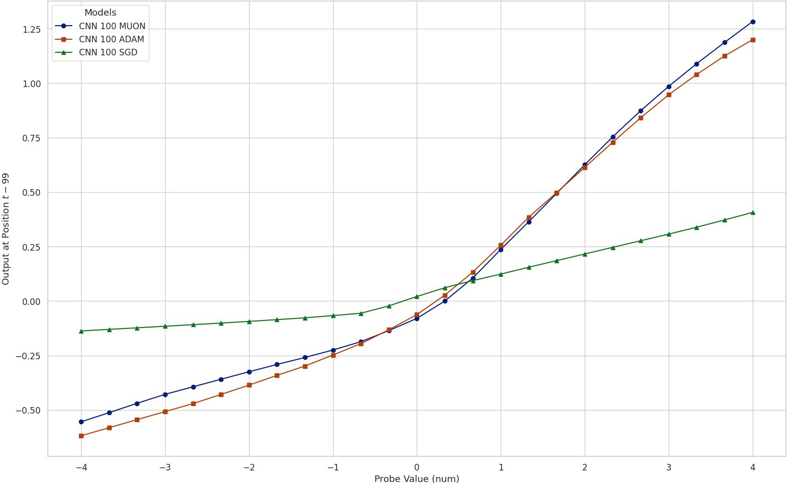
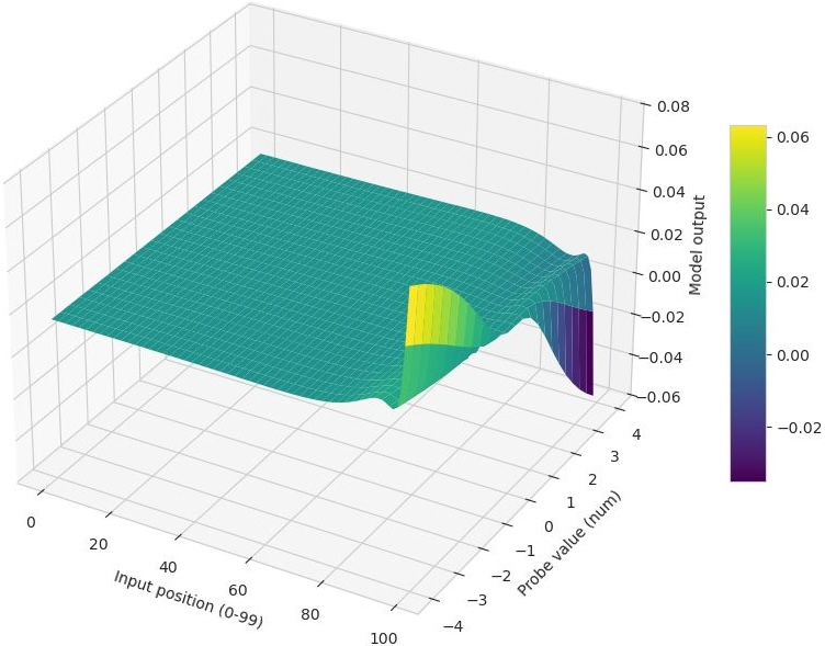
- Impulse response: They changed one input (a specific day in the past) and watched how the prediction moved. This shows how sensitive the model is to specific past days and to big vs. small shocks.
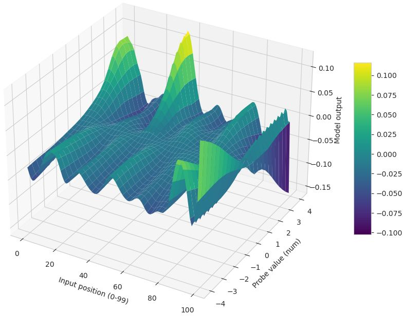
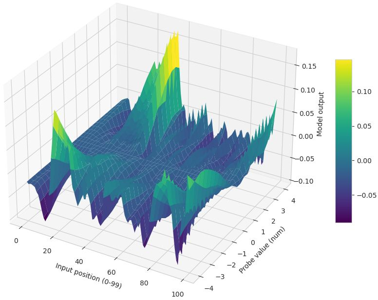
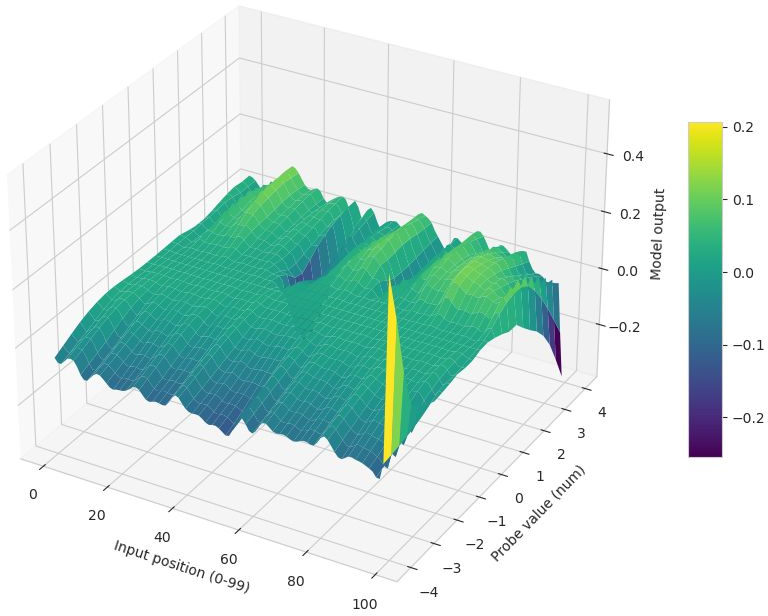
- Difference surfaces: They compared two models’ outputs directly across many inputs. If the differences are “lumpy” (not a simple flat shift), the models are truly doing different things.
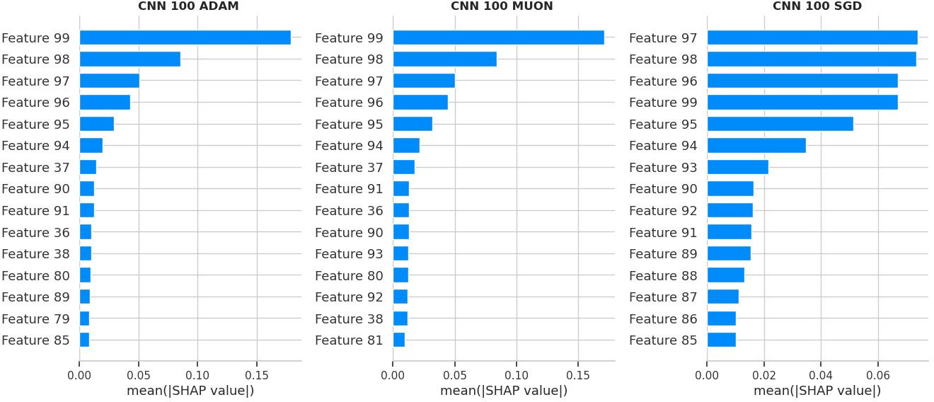
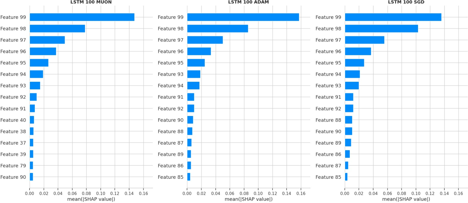
- SHAP feature importance: A method that estimates how much each input day (lag) contributes to the prediction—like splitting “credit” among inputs.
- Ensembling: They averaged predictions from different models. If the average does better, it means the models are catching different pieces of the pattern.
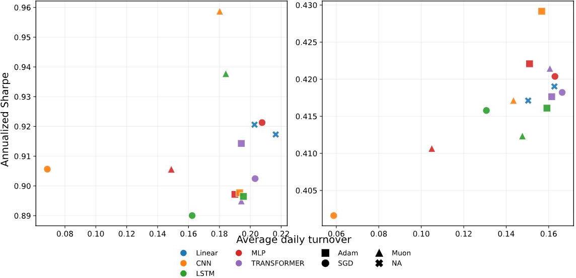
They also checked how these predictions would be used in practice: ranking stocks by predicted volatility and seeing how that affects “turnover” (how often you trade) and “Sharpe ratio” (a simple score for return per unit of risk).
What did they find?
Here are the key takeaways:
- Same score, different behavior:
- Many models—simple and complex—got nearly identical test error. Even after careful tuning, there was a “leaderboard tie.”
- But under the hood, the models’ “rules” were different. Some formed simple, almost straight-line reactions to past volatility; others showed more complicated, curved reactions (like dampening big spikes).
- The optimizer acts like a hidden preference (an “implicit prior”):
- SGD (one optimizer) tended to produce simpler, smoother rules that relied more on very recent days.
- Adam and Muon (other optimizers) often produced more complex, non‑linear rules and sometimes paid attention to longer histories.
- This happened across different architectures, so the choice of optimizer, not just the model type, really mattered.
- The differences are systematic, not random:
- When they compared two optimizers’ models directly, the difference wasn’t a flat line—it had structure—showing the models weren’t just scaled versions of each other.
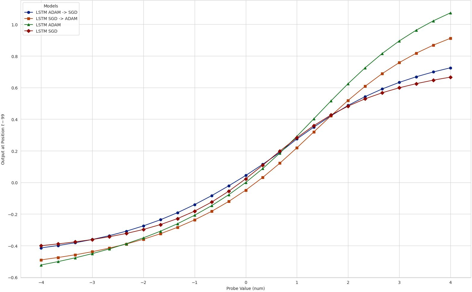
- Swapping optimizers mid-training pulled the model toward the “style” typical of the new optimizer. For example, starting with a complex Adam-trained model and switching to SGD made the model simplify.
- Combining models helped:
- Averaging predictions from models trained with different optimizers beat each model alone. This means each model was finding some unique information the others missed.
- Real-world impact: same Sharpe, very different turnover
- When used to build portfolios, models with similar Sharpe ratios produced very different turnover (how often you trade). In some cases, turnover differed by nearly 3×.
- More turnover means more trading costs. So even if two models have the same “accuracy,” one might be far more expensive to use.
What’s going on under the hood? A helpful picture is the “loss landscape,” which you can imagine as hills and valleys representing how good or bad the model is. SGD tends to settle in wide, shallow valleys (flatter regions)—leading to simpler rules. Adam and Muon can move into narrow, steep valleys (sharper regions)—leading to more complex rules. Training naturally balances near a kind of “edge of stability,” and different optimizers navigate that edge differently.
Why is this important?
- Tied test scores can be misleading: In low‑signal areas like finance, many models can look equally good by a single error number, but they behave differently in ways that matter for decisions.
- The optimizer is part of the model: It doesn’t just speed up training. It nudges the model toward certain kinds of rules—simpler vs. more complex, short‑term vs. longer‑term focus.
- Choose by behavior, not just a number: If your goal is a strategy that trades less (lower turnover), you might favor the optimizer that produces smoother, more stable rankings. If you want sensitivity to certain patterns (like dampening big shocks), you might choose another.
- Practical bottom line: In finance, small differences in “style” can change costs and risks. So model selection should look beyond a single score and include how the model behaves and what that means for real trading.
In one sentence
When many models tie on accuracy, the way you train them quietly decides what kind of rule they learn—and that choice can change how much you trade and how usable your strategy is; in finance, the optimizer is part of the model.
Knowledge Gaps
Below is a single, consolidated list of the paper’s unresolved knowledge gaps, limitations, and open questions. Each item is phrased to be concrete and actionable for future research.
- [Scope/Generalizability] Test whether optimizer-driven functional divergence persists beyond S&P 500 daily volatility (e.g., other equities, international markets, fixed income, FX, commodities, crypto; alternative frequencies such as intraday or weekly).
- [Scope/Targets] Extend from one-step-ahead point forecasts of log-variance to multi-horizon forecasting, interval/probabilistic forecasts (e.g., CRPS, log-likelihood), and alternative targets (e.g., realized kernels, bipower variation, implied volatility).
- [Benchmarks] Compare against specialized econometric volatility models (e.g., GARCH family, HAR-RV, MIDAS, realized-kernel models) to validate that the “leaderboard tie” and functional divergence hold against domain-strong baselines.
- [Feature Set] Assess whether the optimizer-as-prior effect survives with richer inputs (returns, volumes, order-flow proxies, macro/news features, sector/market factors) rather than lagged volatility alone.
- [Cross-sectional Structure] Clarify and test whether the model is pooled across stocks or trained per-asset; quantify heterogeneity in optimizer effects across sectors, firm characteristics, and liquidity tiers.
- [Nonstationarity] Evaluate robustness under regime-aware evaluation (rolling/retraining windows, pre/post-crisis splits, and explicit stress-regime segments) and assess how functional divergence evolves over time.
- [Normalization/Preprocessing] Systematically vary normalization schemes (global vs rolling z-scores), lookback window lengths, and target transforms (log vs variance) to measure sensitivity of functional divergence.
- [Data Quality/Labels] Examine the impact of volatility measurement noise (Garman–Klass vs alternatives; microstructure contamination) on optimizer-induced differences; test denoising or noise-robust training.
- [Metrics Beyond NMSE] Incorporate calibration and density-based metrics (e.g., likelihood, coverage of prediction intervals) and rank-based metrics to probe whether ties persist beyond NMSE/R2.
- [Quantifying “Rashomon”] Provide formal power analyses and confidence intervals for “ties,” including multiple-comparisons corrections, to quantify how much performance must differ to be practically distinguishable.
- [Functional-Difference Quantification] Move beyond visual surfaces to define numerical distances between learned functions (e.g., integrated squared differences over a data-weighted input distribution, Jacobian norms, CCA of hidden states) and test significance of these distances.
- [In-support Sensitivity] Recompute impulse-response and difference surfaces conditioned on the empirical data manifold (e.g., conditional interventions, partial dependence with realistic covariation) rather than setting all other lags to their mean.
- [Attribution Robustness] Validate SHAP-based lag-importance under strong autocorrelation/collinearity across lags; compare with conditional SHAP, Integrated Gradients, or time-series–aware attribution to ensure stability of conclusions.
- [Optimizer Breadth] Expand optimizer coverage (SGD+momentum/Nesterov, AdamW, RMSProp, Adagrad, AdaBelief, AdaFactor, Lion, Shampoo, K-FAC/second-order) to map the diversity of implicit priors and identify which update geometries drive which function classes.
- [Hyperparameter Breadth] Tune optimizer hyperparameters beyond learning rate and weight decay (e.g., momentum, Adam β1/β2, ε, decoupled weight decay, learning-rate schedules) and quantify their impact on function selection.
- [Batch Size/Noise] Vary batch size and gradient noise to test predicted effects from Edge-of-Stability (EoS) theory on selected minima and functional complexity; document whether optimizer differences widen or shrink with batch-size changes.
- [Training Length/Stopping] Examine how training duration (pre- vs post-EoS horizon), early stopping, and schedule shape (warmups, cosine decay) affect the emergence of functional divergence.
- [Initialization/Normalization] Test robustness to different initialization schemes (e.g., Xavier/He, scaled orthogonal) and architectural normalizations (batch/layer norm), and whether these interact with optimizer-induced priors.
- [Curvature Measurement Robustness] Provide methodological details and stability checks for Hessian eigenvalue estimation (sampling strategy, variance across seeds/layers); assess whether sharpness-function complexity links persist under alternative curvature proxies.
- [Mechanistic Theory] Develop a formal theory linking optimizer geometry and preconditioning to specific temporal weighting patterns and nonlinearity (e.g., why sharper minima coincide with long-memory utilization or dampening mechanisms).
- [Intervention Design] Extend optimizer-swap experiments with controlled preconditioning ablations (e.g., normalized gradients only), explicit noise injections, and matched learning rates/step norms to isolate causal levers.
- [Decision-level Costs] Incorporate realistic transaction-cost, slippage, and market-impact models to translate turnover dispersion into net performance differences; report capacity and robustness under costs.
- [Portfolio Construction] Stress test decision-level findings across portfolio rules (deciles vs quintiles, continuous risk budgets), rebalance frequencies, and constraints (e.g., sector neutrality), and assess statistical significance of Sharpe/turnover gaps.
- [Turnover Control] Explore training objectives that explicitly penalize instability/turnover (e.g., rank or temporal smoothness penalties) to see if optimizer-induced priors can be replaced with explicit regularization aligned with implementability.
- [Ensembling Strategy] Systematically design ensembles that exploit optimizer diversity (e.g., stacking, diversity-aware weighting) and evaluate trade-offs between error reduction and turnover/signal stability.
- [Regime-conditioned Functions] Relate learned functional features (e.g., quarterly lag emphasis, nonlinear dampening) to economic mechanisms via event studies (earnings cycles, macro announcements) to validate interpretability claims.
- [Reproducibility] Release code and exact preprocessing details; specify train/validation/test splits, pooling strategy, lookback length, scaling protocol, batch sizes, and all hyperparameters to enable independent replication.
- [External Validity] Investigate whether functional divergence narrows with larger data (e.g., longer histories, higher-frequency realized measures) or with transfer/pretraining approaches, and whether more data resolves underspecification.
Practical Applications
Immediate Applications
The paper’s findings enable several deployable practices that treat the optimizer as a controllable inductive prior and evaluate models beyond scalar loss, especially in low-signal, high-noise time series.
- Optimizer-aware model selection for trading
- Sectors: Finance (asset management, quant trading, risk)
- What it enables: Choose optimizers to match implementation constraints: SGD for simpler, more stable forecasts with lower turnover; Adam/Muon for more reactive forecasts when rapid adaptation is prioritized.
- Tools/workflows: Decision-aware validation that reports a Sharpe–turnover frontier; routine impulse-response maps and lag-wise SHAP attributions; optimizer sweeps in hyperparameter search.
- Assumptions/dependencies: Paper’s effects are shown on S&P 500 volatility forecasting; turnover differential depends on strategy design, transaction cost model, and broker microstructure.
- Optimizer-diverse ensembling to reduce error and model risk
- Sectors: Finance (quant research, portfolio construction)
- What it enables: Ensemble across optimizer-induced solutions (e.g., Adam/SGD/Muon) to exploit complementary signal and lower NMSE versus any constituent; diversify “model-multiplicity” risk.
- Tools/workflows: Lightweight stacking/averaging libraries that treat optimizer choice as an ensemble dimension; monitoring of error correlation across members.
- Assumptions/dependencies: Gains rely on imperfectly correlated residuals; added latency/compute for multiple model runs.
- Transaction-cost-aware deployment via turnover targeting
- Sectors: Finance (execution, portfolio management)
- What it enables: Select optimizer to meet turnover budgets; deploy SGD-trained models when costs/capacity constraints dominate; switch to adaptive optimizers in stress regimes requiring reactivity.
- Tools/workflows: Turnover budgeting in backtests; optimizer-switch playbooks conditioned on market regimes; live turnover dashboards.
- Assumptions/dependencies: Requires stable cost estimates; regime detection must be reliable to avoid whipsaw.
- Model risk governance: optimizer stress tests and disclosures
- Sectors: Finance (model validation, compliance), Policy (supervision)
- What it enables: Add “optimizer sensitivity” to model validation packs—report functional diagnostics (difference surfaces, lag attributions) and decision metrics (turnover stability) alongside NMSE.
- Tools/workflows: Validation checklists, audit trails logging optimizer configuration and curvature statistics; challenger models trained with alternative optimizers.
- Assumptions/dependencies: Organizational buy-in to extend validation beyond loss metrics; compute budget for challenger models.
- MLOps monitoring of curvature/sharpness and stability
- Sectors: Software/MLOps for quantitative systems
- What it enables: Track proxies for maximum Hessian eigenvalue and edge-of-stability behavior to anticipate instability; operationalize optimizer swaps to simplify or complexify functions on demand.
- Tools/workflows: EoS monitors using efficient sharpness proxies (e.g., power iteration, Fisher approximations), scheduled “optimizer intervention” jobs.
- Assumptions/dependencies: Exact Hessian is expensive; must use approximations that correlate with decision stability; monitor noise from online training.
- AutoML with decision-aware objectives
- Sectors: Software (AutoML), Finance (research platforms)
- What it enables: Include optimizer choice and weight decay/learning-rate grids in search; optimize for composite objectives (e.g., NMSE subject to turnover caps).
- Tools/workflows: Extensions to Optuna/Weights & Biases that track decision-level KPIs and functional diagnostics; Pareto front reporting.
- Assumptions/dependencies: Requires clear, quantifiable downstream constraints; careful validation splits to avoid overfitting to decision metrics.
- Interpretability-first functional diagnostics in low-signal domains
- Sectors: Academia, Finance, Energy, Operations
- What it enables: Standardize impulse-response and SHAP lag profiles to understand temporal dependence learned under different optimizers, even when losses tie.
- Tools/workflows: “Functional divergence explorer” notebooks/dashboards to compare response surfaces and difference maps across checkpoints/optimizers.
- Assumptions/dependencies: SHAP assumptions and computational cost; diagnostics must be tailored for sequence inputs and log-variance targets.
- Stability-reactivity tuning for operational forecasts
- Sectors: Healthcare (ICU alarms), Energy (demand/price), Supply chain (inventory), IoT
- What it enables: Use optimizer choice to tune sensitivity vs stability in alerts/controls (e.g., SGD for fewer false alarms; adaptive methods for faster reaction to regime shifts).
- Tools/workflows: Dual-model deployments with optimizer-based “knobs”; service-level objective (SLO) dashboards emphasizing alert churn/switching frequency.
- Assumptions/dependencies: Applicability relies on presence of underspecification and similar loss ties; domain-specific cost of switching/alerts must be quantified.
- Robo-advisors and retail trading bots: cost-aware rebalancing
- Sectors: Finance (retail wealth, crypto)
- What it enables: Reduce churn and fees by favoring optimizers that induce stable rankings and lower turnover for rebalance schedules.
- Tools/workflows: Backtests exposing turnover and fee drag by optimizer; user-facing “stability vs responsiveness” slider mapping to optimizer choice.
- Assumptions/dependencies: Broker fee structure, tax implications, and liquidity constraints; smaller accounts more sensitive to fees.
- Replicable academic evaluation protocols
- Sectors: Academia (financial ML, econometrics)
- What it enables: Publish benchmarks that report both scalar error and functional/decision metrics; require optimizer sweeps and optimizer-difference surfaces for credible claims.
- Tools/workflows: Public code templates; dataset cards documenting survivorship-bias-free construction and evaluation splits.
- Assumptions/dependencies: Community standards and compute budgets for multi-optimizer experiments.
Long-Term Applications
The study motivates new algorithms, standards, and infrastructure that treat optimization geometry as an explicit design lever for decision stability and implementability.
- Optimizers that internalize economic costs (e.g., turnover penalties)
- Sectors: Finance (strategy design), Software (optimizer R&D)
- What it enables: New optimizers or preconditioners that bias toward smoother decision boundaries and stable rankings under equivalent predictive loss.
- Tools/products: “Turnover-aware Adam/SGD” or matrix-aware methods with controllable sharpness/complexity; differentiable approximations of rank stability.
- Assumptions/dependencies: Requires reliable proxies linking sharpness/geometry to turnover; careful integration to avoid degrading forecast accuracy.
- Meta-controllers for regime-aware optimizer scheduling
- Sectors: Finance (systematic macro/equities), Energy/Operations
- What it enables: Switch or blend optimizers online based on detected regime (stress vs normal) to trade off responsiveness and stability dynamically.
- Tools/products: Bandit/RL-based scheduler over optimizers; guardrails for stability and risk limits.
- Assumptions/dependencies: Robust regime detection; safe transitions without introducing instability.
- Formal links between curvature and decision metrics
- Sectors: Academia, Finance (risk), Policy (standards)
- What it enables: Theory and empirical tests connecting sharpness/EoS to portfolio turnover, rank reversals, and capacity; calibration rules for safe operating points.
- Tools/workflows: New evaluation benchmarks and stylized-model analyses; certified bounds on decision volatility given optimizer settings.
- Assumptions/dependencies: May vary across architectures, datasets, and market conditions; requires multi-market validation.
- Decision-aware AutoML and differentiable utilities
- Sectors: Software (AutoML), Finance
- What it enables: Optimize end-to-end utility (e.g., expected net returns after cost) with surrogate gradients for turnover and slippage; choose optimizer/architecture jointly.
- Tools/products: AutoML that searches over optimizers, regularization, and ensembling under multi-objective constraints; Pareto-efficient policy suggestion.
- Assumptions/dependencies: Differentiable surrogates must correlate with realized implementation costs; risk of gaming metrics.
- Multiplicity-aware regulatory standards
- Sectors: Policy/Regulation (model risk, market integrity)
- What it enables: Require “optimizer stress tests” and multiplicity disclosures for ML-based trading/risk models; include decision stability metrics in model approval.
- Tools/products: Supervisory guidance updates (e.g., extensions to SR 11-7 for ML), audit templates, benchmark suites.
- Assumptions/dependencies: Regulatory capacity and consensus that optimizer choice materially affects outcomes; industry feedback loops.
- Production-grade curvature monitoring and proxies
- Sectors: Software/MLOps, Finance, Healthcare
- What it enables: Low-overhead online sharpness proxies and EoS tracking for live models; early warnings and automatic mitigation (e.g., learning-rate/optimizer adjustments).
- Tools/products: Agents that estimate λ_max proxies with randomized tests; integration into CI/CD for models.
- Assumptions/dependencies: Proxy fidelity across architectures; acceptable overhead at production latencies.
- Optimizer-heterogeneous model marketplaces
- Sectors: Finance (data/model vendors), Software
- What it enables: Distribute model families differentiated by optimizer-induced behavior (stable vs reactive variants), letting clients select per cost/latency profile.
- Tools/products: Catalogs with functional and decision metrics; SLAs for turnover and stability.
- Assumptions/dependencies: Clear demand segmentation; standardized reporting for comparability.
- Cross-domain stability engineering via optimizer priors
- Sectors: Healthcare (clinical decision support), Robotics/Autonomy, Smart grids
- What it enables: Design learning systems whose control/alert smoothness is governed by optimizer geometry rather than post-hoc smoothing; mitigate alarm fatigue or actuator wear.
- Tools/products: Stability-calibrated optimizers for safety-critical time series; certification frameworks.
- Assumptions/dependencies: Validation in each domain’s safety regime; mapping between decision volatility and optimizer settings.
- Bayesian and causal treatments of optimizer as prior
- Sectors: Academia
- What it enables: Treat optimizer choice as an implicit prior in Bayesian model averaging or causal analyses of decision rules; incorporate optimizer diversity into posterior ensembles.
- Tools/workflows: Posterior-weighted ensembles indexed by optimizer; causal diagnostics for decision multiplicity.
- Assumptions/dependencies: Formalizing the optimizer–prior mapping; computational overhead.
- Education and workforce development
- Sectors: Academia, Industry training
- What it enables: Curricula that elevate optimizer selection to a first-class design choice in low-SNR forecasting; labs on impulse-response, SHAP lag attributions, EoS behavior.
- Tools/workflows: Open-source teaching kits; benchmark datasets with survivorship-bias controls.
- Assumptions/dependencies: Adoption by programs; sustained maintenance of teaching resources.
Glossary
- Adam: An adaptive optimization algorithm that uses estimates of first and second moments of gradients to adjust learning rates per parameter. "Many empirical studies default to common baselines, such as Adam, without investigating the implication of optimizer choice \citep{gu2020empirical, chen2024deep}."
- Ambiguity decomposition: A result in ensemble learning showing that an ensemble can outperform its members when their errors are diverse (not perfectly aligned). "— by the ambiguity decomposition \citep{NIPS1994_b8c37e33} — the predictors must disagree on a non-negligible set of inputs, i.e., their errors are not perfectly aligned."
- Autocorrelation: The correlation of a time series with its own past values. "daily volatility exhibits strong autocorrelation and clustering"
- Catapult effect: A training instability where SGD can be repelled from sharp minima near stability limits, causing rapid trajectory shifts. "echoing the catapult effect of SGD at instability highlighted by \cite{andreyev2025edgestochasticstabilityrevisiting}."
- CRSP: The Center for Research in Security Prices, a key database for U.S. equity data. "constructed from CRSP (see Appendix \ref{app:choosing_dataset} and \ref{app:dataset_analysis} for further details)."
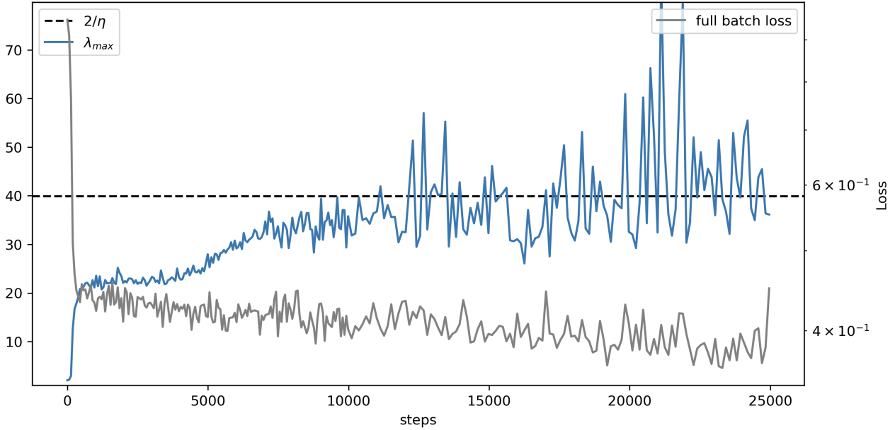
- Curvature: The sharpness of the loss landscape, often quantified by the Hessian’s eigenvalues. "during SGD training the curvature (top Hessian eigenvalue ) increases until it reaches the stability threshold and subsequently stabilizes."
- Difference surface: A surface that visualizes pointwise output differences between two models across an input grid. "The difference surface $D = \hat{y}_{\text{Muon} - \hat{y}_{\text{Adam}$ plotted for LSTM (left), CNN (middle), and Transformer (right)."
- Edge of (Stochastic) Stability (EoSS): A regime where training operates near the stability boundary defined by step size and curvature. "First, we confirm that financial neural networks exhibit Edge of (Stochastic) Stability (EoSS) dynamics"
- Ensemble predictor: A model that aggregates multiple predictors (e.g., by averaging) to reduce error via diversity. "Finally, to assess whether estimation errors are correlated across estimation systems, we construct an ensemble predictor"
- Garman–Klass estimator: A range-based estimator of realized variance derived from OHLC prices. "The target variable is realized variance, proxied by the Garman--Klass estimator (\citet{0d979ce1-e68e-3a44-a15a-4554e7fd21ca}) computed from daily high (), low (), open (), and close () prices:"
- Hessian eigenvalue (maximum): The largest eigenvalue of the Hessian matrix; measures the sharpest curvature direction of the loss. "we compute the maximum Hessian eigenvalue () at convergence for both CNN and MLP models."
- Implicit prior: An inductive bias introduced by the optimization process rather than explicit regularization or model design. "Optimizer as implicit prior."
- Impulse response: The model’s output response when a single input dimension (lag) is perturbed while others are held fixed. "We define the impulse response as the model output when the -th lag is set to value and all other inputs are held at their mean (zero):"
- Inductive bias: The set of assumptions that guide a learning algorithm toward particular solutions among many fits. "optimization acts as a consequential source of inductive bias"
- LASSO: A linear regression technique with L1 regularization that performs variable selection and shrinkage. "linear baselines (OLS/LASSO)"
- Log-variance: The natural logarithm of variance; used as a target transformation to stabilize training. "Models are trained to predict the log-variance, using a lookback window of past daily volatilities."
- Matrix-aware optimizer: An optimizer that leverages matrix-structured information (e.g., curvature) to shape updates. "Muon \citep{jordan2024muon}, a recent matrix-aware optimizer designed for high-dimensional training dynamics."
- Microstructure effects: Short-horizon market frictions and dynamics arising from trade execution, tick sizes, and bid-ask mechanics. "short-horizon volatility dynamics driven by microstructure effects, order flow, and volatility clustering \citep{engle1982autoregressive}"
- Muon: A recent matrix-aware optimization algorithm tailored for high-dimensional training dynamics. "The LSTM (trained with Muon) exhibits a curved decision boundary, indicating distinct non-linear sensitivity to volatility shocks at specific lags."
- NMSE (Normalized Mean Squared Error): Mean squared error scaled (e.g., by variance) to enable comparability across settings. "Because standard metrics such as Normalized Mean Squared Error (NMSE) or are insufficient to distinguish between models in low-signal settings"
- OLS (Ordinary Least Squares): A basic linear regression estimator minimizing squared residuals. "OLS and LASSO achieve error levels statistically indistinguishable from even the most complex Transformer models."
- Optuna: An automated hyperparameter optimization framework. "we perform a rigorous hyperparameter optimization for every architecture--optimizer pair using the Optuna framework \citep{akiba2019optunanextgenerationhyperparameteroptimization}."
- Order flow: The sequence and size of buy/sell orders that influence short-term price dynamics. "short-horizon volatility dynamics driven by microstructure effects, order flow, and volatility clustering \citep{engle1982autoregressive}"
- Out-of-sample performance: Evaluation on held-out data not used during training or validation. "In financial time series forecasting, substantially different predictors often achieve indistinguishable out-of-sample performance under standard loss metrics."
- Overparameterized regime: A setting where the model has more parameters than constraints, allowing many near-equivalent fits. "In overparameterized regimes, training dynamics play a central role in selecting many compatible solutions \citep{wilson2017marginal, zou2021adam}."
- Preconditioning: A transformation of gradient updates to normalize curvature and improve optimization stability. "Adaptive methods (like Adam) effectively ``flatten'' the optimization landscape via preconditioning, allowing the optimizer to stably descend into narrow valleys (high original curvature) that are inaccessible to SGD."
- Predictive multiplicity: The existence of multiple models with similar aggregate error but different predictions/behaviors. "a phenomenon related to underspecification and predictive multiplicity (see Appendix~\ref{app:further_work})."
- Rashomon Effect: The observation that many disparate models can achieve similar predictive performance on a task. "This phenomenon has been formalized as underspecification \citep{damour2020underspecification}, extending Breiman's Rashomon Effect \citep{breiman2001statistical}."
- Realized variance: An ex-post measure of variance computed from observed price data within a period. "The target variable is realized variance, proxied by the Garman--Klass estimator (\citet{0d979ce1-e68e-3a44-a15a-4554e7fd21ca})"
- Receptive field (effective receptive fields): The range of input lags or positions that significantly influence a model’s output. "temporal attributions uncover optimizer-dependent ``effective receptive fields''"
- SHAP (SHapley Additive exPlanations): A game-theoretic method for attributing feature contributions to model predictions. "we employ SHapley Additive exPlanations (SHAP) \citep{lundberg2017unifiedapproachinterpretingmodel}."
- Sharpe ratio: A risk-adjusted performance metric defined as mean return over return volatility. "Across both quintiles, Sharpe ratios are broadly similar across models"
- Signal-to-noise ratio: The relative magnitude of informative signal versus random noise in data. "a task characterized by a low signal-to-noise ratio"
- Stability threshold: The step-size–curvature boundary beyond which gradient updates become unstable. "reaches the stability threshold "
- Survivorship bias: Bias arising from analyzing only entities that remain over time, excluding those that dropped out. "We build a survivorship-bias-free dataset of S{paper_content}P 500 constituents spanning 2000--2024, constructed from CRSP"
- Turnover: The rate at which a portfolio’s holdings change, often linked to trading costs. "portfolio turnover varies substantially despite comparable risk-adjusted performance"
- Underspecification: A situation where multiple distinct models fit observed data equally well under chosen metrics. "Neural networks applied to financial time series operate in a regime of underspecification, where model predictors achieve indistinguishable out-of-sample error."
- Update geometry: The direction and scaling structure of an optimizer’s parameter updates in the loss landscape. "We contrast three optimization methods that differ in update geometry and implicit regularization."
- Volatility clustering: The empirical tendency for high (or low) volatility to persist over time. "short-horizon volatility dynamics driven by microstructure effects, order flow, and volatility clustering \citep{engle1982autoregressive}"
- Volatility-managed portfolio: A strategy that scales exposures based on forecasted volatility to target risk. "We construct volatility-managed portfolios and report the resulting Sharpe--Turnover frontier in Figure~\ref{fig:sharpe_turnover_q1q5}."
- Weight decay: L2 regularization applied during optimization to penalize large weights. "performing optimizer-specific hyperparameter searches (learning rate, weight decay) for every architecture--optimizer pair."
Collections
Sign up for free to add this paper to one or more collections.