Bridging Physically Based Rendering and Diffusion Models with Stochastic Differential Equation
Abstract: Diffusion-based image generators excel at producing realistic content from text or image conditions, but they offer only limited explicit control over low-level, physically grounded shading and material properties. In contrast, physically based rendering (PBR) offers fine-grained physical control but lacks prompt-driven flexibility. Although these two paradigms originate from distinct communities, both share a common evolution -- from noisy observations to clean images. In this paper, we propose a unified stochastic formulation that bridges Monte Carlo rendering and diffusion-based generative modeling. First, a general stochastic differential equation (SDE) formulation for Monte Carlo integration under the Central Limit Theorem is modeled. Through instantiation via physically based path tracing, we convert it into a physically grounded SDE representation. Moreover, we provide a systematic analysis of how the physical characteristics of path tracing can be extended to existing diffusion models from the perspective of noise variance. Extensive experiments across multiple tasks show that our method can exert physically grounded control over diffusion-generated results, covering tasks such as rendering and material editing.

Paper Prompts
Sign up for free to create and run prompts on this paper using GPT-5.
Top Community Prompts
Explain it Like I'm 14
Overview
This paper connects two different ways of making realistic images:
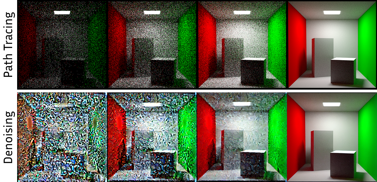
- Physically Based Rendering (PBR), especially a method called path tracing, which simulates how light bounces to create lifelike pictures but needs lots of time to remove “grainy” noise.
- Diffusion models (like Stable Diffusion), which are AI systems that start with random noise and slowly “clean” it into a detailed image from a prompt.
The big idea is that both systems move from noisy images to clean images. The paper builds a shared, simple mathematical story (a kind of “step-by-step cleaning process”) that explains both in the same way. Then it uses that shared story to control things like shine, gloss, and lighting in AI-generated images using physical rules from PBR.
Key Objectives and Questions
The authors aim to:
- Build one unified model that describes how both path tracing and diffusion models turn noise into a clean image.
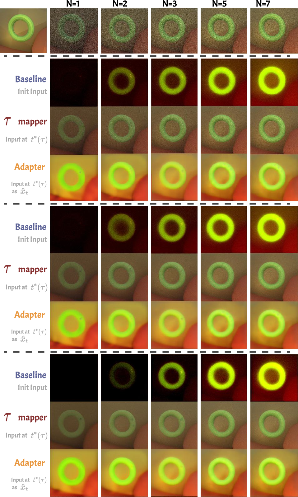
- Create a way to match “how noisy” a path-traced image is to the “right moment” inside a diffusion model’s denoising steps, so the diffusion model can take over and clean it properly.
- Use this connection to control material properties (like glossiness vs. dullness) and lighting in diffusion-generated images based on physical behavior, not just prompts.
Methods (Explained Simply)
Think of image making like cleaning a foggy photo:
- In path tracing (PBR), you take many random samples (like lots of tiny snapshots of light) to reduce grainy noise. Fewer samples = more noise; more samples = cleaner image. Over time, the picture becomes clearer.
- In diffusion models, you start with noise and repeatedly apply steps that remove noise to reveal a clean image.
The authors show these two “cleaning” processes can be written as the same kind of step-by-step rule called a stochastic differential equation (SDE). Here’s an everyday analogy:
- Imagine every step wipes away a little more fog. In path tracing, taking more samples wipes away fog. In diffusion, each denoising step wipes away fog. The SDE is the recipe for how much fog gets wiped at each step.
Key pieces they introduce:
- Variance time (called τ): a simple number that measures “how noisy” a path-traced image is. Big τ = lots of noise (few samples). Small τ = less noise (many samples).
- A mapping between τ and the diffusion model’s timestep t: this tells the diffusion model where to start its cleaning, based on how noisy the path-traced image is.
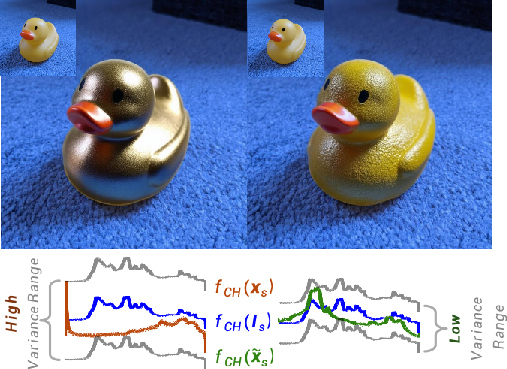
- Shared noise for materials: they treat diffuse (soft, matte) and specular (shiny, mirror-like) parts as driven by the same randomness, which lets them explain why shiny parts are noisier and settle later.
They match noise levels using signal-to-noise ratio (SNR), which is just a way to compare “how strong the image signal is” versus “how much noise is left.”
Main Findings and Why They Matter
Here are the main results and their importance:
- A single “cleaning” rule fits both worlds: The Monte Carlo SDE (MC-SDE) they derive for path tracing matches the reverse SDE used by diffusion models. This means both are truly two views of the same kind of process.
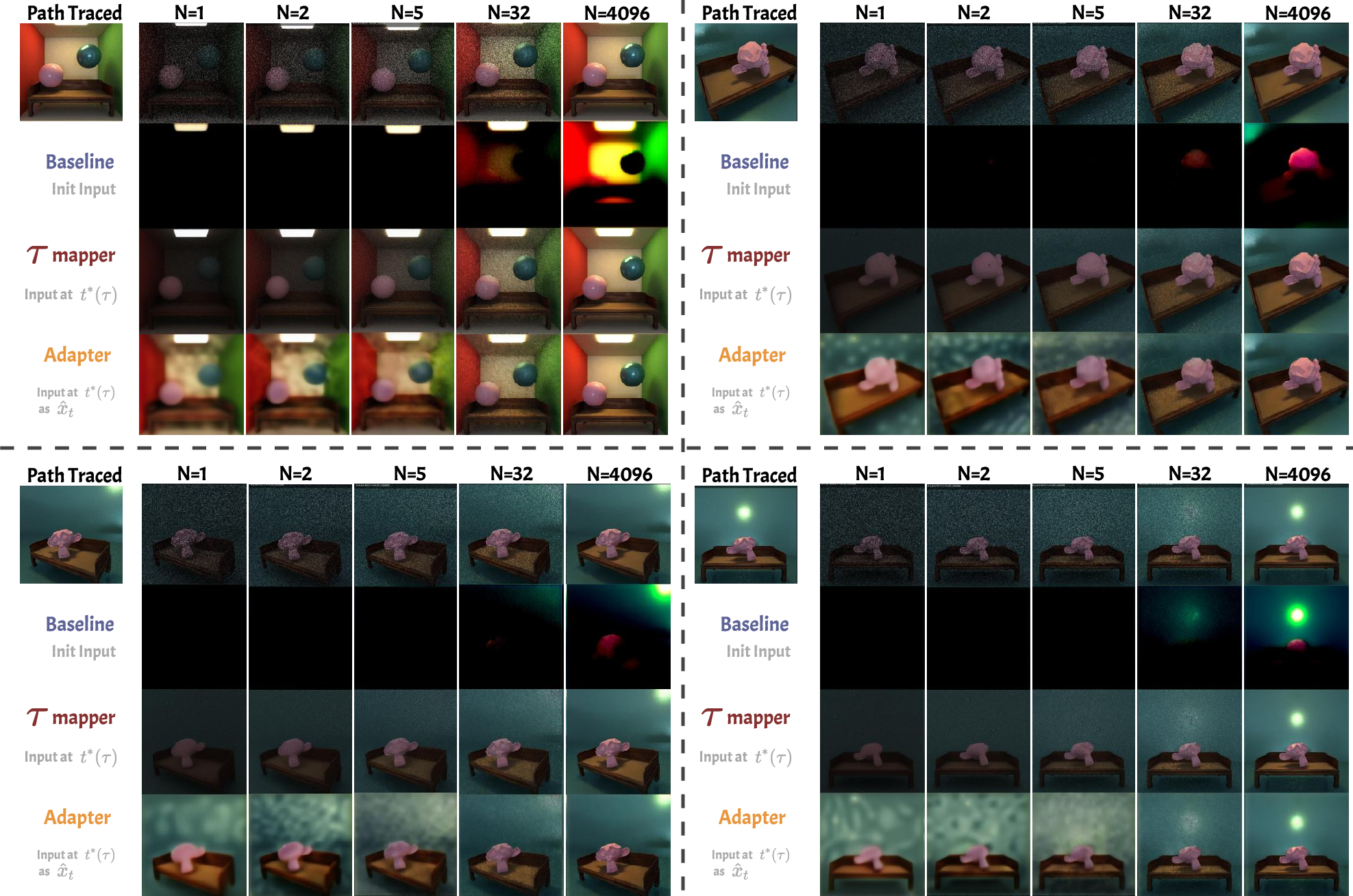
- Correct starting point for cleaning: They give a formula to map a path-traced image’s sample count (how many rays you traced) to the right diffusion timestep. With this, a pre-trained diffusion model can “take over” a noisy render and clean it into a realistic image instead of getting confused.
- Shiny things settle later: Specular (shiny) surfaces have much higher noise than diffuse ones. In both path tracing and diffusion, shiny details naturally become correct later in the denoising process. Knowing this, you can control materials more precisely by adjusting early vs. late denoising steps.
- Better color and contrast with a tiny adapter: They add a lightweight adapter that reshapes the noise distribution of path-traced inputs to what the diffusion model expects, improving color range and accuracy.
- Practical demos: They show:
- Diffusion models can denoise low-sample path-traced images well when you start at the matched timestep.
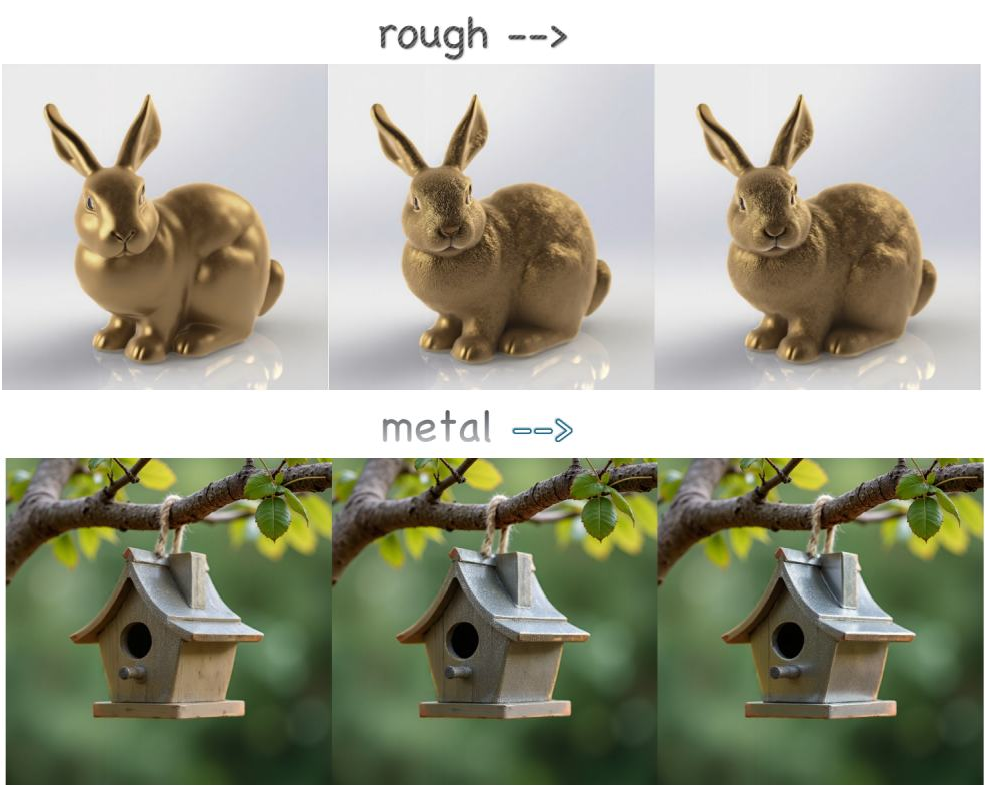
- You can tune materials (metallic vs. roughness) in diffusion images by giving more “attention” to high-frequency (shiny) features early and letting them taper off later, producing smooth and realistic control.
Why this matters: You get the flexibility of diffusion models (easy, prompt-driven generation) plus the physical control of PBR (accurate shading and material behavior). This opens the door to more realistic, controllable AI-generated images.
Implications and Impact
- For artists and designers: Easier control of gloss, highlights, and material properties inside diffusion models, guided by physical rules—not just vague prompts.
- For games and movies: Faster workflows—start with a noisy render and let a diffusion model clean it, or edit materials consistently across shots.
- For research: A shared language between rendering and generative models makes it simpler to combine the strengths of both, potentially improving realistic image generation, editing, and even inverse rendering (figuring out materials from photos).
In short, this paper shows that physics-based rendering and AI diffusion models are two sides of the same “noise-to-clean” coin. By connecting them, we can get both realism and control in a single, powerful image-making pipeline.
Knowledge Gaps
Knowledge gaps, limitations, and open questions
The following list summarizes what is missing, uncertain, or left unexplored in the paper, formulated as concrete, actionable gaps for future research:
- Clarify the scope and validity of the CLT/Gaussian assumption for path tracing noise, especially under heavy-tailed distributions caused by specular microfacets, visibility discontinuities, caustics, and delta BSDFs where finite second moments may not hold.
- Extend the MC-SDE derivation beyond single-bounce/direct illumination to the full path integral with multiple bounces, next-event estimation, MIS, Russian roulette, and delta distributions, and characterize the resulting drift/diffusion terms.
- Analyze how stratified sampling, QMC/low-discrepancy sequences, or correlated sampling techniques alter the noise model and whether the MC-SDE mapping remains valid under non-i.i.d. sampling.
- Generalize the “shared noise source” assumption (same random draw for diffuse/specular) to realistic BSDF-specific sampling strategies and quantify the impact on the covariance structure and specular/diffuse dominance claims.
- Provide a principled method to estimate per-pixel variance-time τ (or spp N) directly from a noisy path-traced image, including cases with spatially varying spp (adaptive sampling), instead of requiring known N.
- Develop per-pixel (heteroskedastic) τ→t schedules that account for spatially varying variance and structured noise, rather than a global alignment.
- Replace the heuristic choice N(τ)=τ{-2} and constant A calibration with a learned or statistically justified mapping, and quantify how schedule miscalibration affects fidelity and stability.
- Establish theoretical bounds (error, bias, convergence rates) for the τ→t log-SNR alignment, including sensitivity to the diffusion model’s schedule, latent VAE scaling, and classifier-free guidance strength.
- Validate the specular-late-stabilization claim with rigorous frequency-domain analyses (e.g., PSD, multi-scale metrics), beyond qualitative histograms; quantify the cross-over point where high-frequency content becomes recoverable.
- Quantify how well the Gaussian VE reverse-SDE equivalence holds at low spp (non-asymptotic regimes), where CLT may not approximate the empirical noise distribution.
- Characterize and estimate σ (and Σ for vector components) from path-traced data in practice; specify procedures to compute per-component variances and their dependence on scene, materials, and lighting.
- Investigate robustness of the τ→t mapping and adapter across diverse diffusion architectures (e.g., SDXL, pixel-space models), different VAE latents, and varying noise schedules (VP, VE, EDM), including stochastic vs. deterministic samplers.
- Analyze interactions between ControlNet/radiance hints, classifier-free guidance, and the τ→t schedule; determine how external conditioning modifies effective SNR and schedule alignment.
- Provide stronger empirical validation across more scenes/materials/lighting setups (including anisotropic BRDFs, transmission/refraction, subsurface scattering, volumetric media, area/spot lights) to test generality of the bridge.
- Evaluate multi-view and 3D consistency: can the τ→t alignment and material editing yield physically coherent appearance across viewpoints and over geometry/scene changes?
- Incorporate explicit environment lighting estimation/control rather than relying on “lighting embedded in diffusion models”; assess physical plausibility (energy conservation, shadow/occlusion consistency).
- Detail the adapter architecture, training protocol, and failure modes; test generalization to out-of-distribution scenes/materials, different renderers, and varying spp ranges; compare with alternative distribution-matching objectives.
- Study the influence of the latent VAE (compression, color gamut, dynamic range) on the noise distribution mapping; propose corrections for HDR content and color calibration to improve physical fidelity.
- Compare against specialized Monte Carlo denoisers and neural renderers; quantify when the diffusion “takeover” is preferable in terms of quality, compute, and wall-clock time.
- Report computational costs (inference time, memory) and end-to-end speed-ups vs. increasing spp in path tracing; assess practical trade-offs.
- Provide quantitative metrics beyond PSNR/SSIM/LPIPS (e.g., reflectance/lighting parameter recovery, highlight placement accuracy, shadow/edge fidelity, spectral/energy consistency) to evaluate “physically grounded control.”
- Formalize how the vector MC-SDE with correlated components (diffuse/specular) maps into diffusion latent dynamics, including cross-channel (RGB) correlations and the effect on color range/contrast.
- Explore training diffusion models with physics-aware priors or schedules derived from MC-SDE (rather than post-hoc alignment) to improve interpretability and low-level control over shading/materials.
- Develop methods to disentangle and explicitly control specular vs. diffuse components in diffusion outputs (beyond attention-weight heuristics), possibly via auxiliary decoders/heads or physically informed latent factorization.
- Address failure cases: scenes with extreme glossiness, sharp caustics, thin geometry, or complex visibility; characterize when the bridge breaks and propose diagnostics or fallback strategies.
- Investigate domain gaps between rendered and photographic data (camera response, tone mapping, noise characteristics) and their impact on τ→t alignment and adapter performance; propose calibration pipelines.
- Study how schedule alignment and material control extend to temporal domains (video) and dynamic lighting/material changes, ensuring temporal consistency.
- Release code, datasets (including the 30-scene adapter training set), and detailed reproducibility notes to enable independent validation and broader benchmarking.
Practical Applications
Immediate Applications
Below are actionable, sector-linked use cases that can be deployed with current tools and the paper’s proposed methods (τ–t mapping, MC–SDE alignment, lightweight adapter, and noise-stage-aware material control).
- Bold: Diffusion “takeover” denoiser for low-spp path-traced images (Software, VFX/CG, Gaming)
- Use case: Replace expensive high-spp path tracing with low-spp renders plus diffusion-based denoising that is physically aligned via the τ→t log-SNR mapping; optionally add the lightweight time-conditioned adapter to match MC noise to diffusion latent noise.
- Tools/products/workflows:
- Plugin for Blender/Cycles, Autodesk Arnold, RenderMan, Unreal/Path Tracer that reads spp N, computes τ=N{-1/2}, maps to diffusion timestep t via the paper’s log-SNR schedule, then runs DDIM/SDXL denoising.
- “MC–Diffusion Adapter” module trained on a small rendered dataset to convert MC noise to diffusion latent noise distribution.
- Assumptions/dependencies:
- Access to a pretrained diffusion model (e.g., Stable Diffusion v1.4/vXL); knowledge of its noise schedule.
- Input carries accurate spp metadata; MC noise distribution is within adapter’s training domain.
- Scenes adhere to CLT assumptions; uniform or compatible sampling strategies; specular-dominant variance typical in PBR scenes.
- Bold: Render-time acceleration and cost reduction (Cloud Rendering, Media & Entertainment)
- Use case: Cut path-tracing spp budgets (e.g., 1–16 spp) and rely on the τ–t mapper plus adapter to obtain near-ground-truth visual quality, lowering GPU-hours and cloud costs.
- Tools/products/workflows:
- “Green Render” pipeline that selects spp targets per shot, runs MC–SDE-aware denoising, and validates quality via PSNR/SSIM/LPIPS gates as in the paper.
- Assumptions/dependencies:
- Quality thresholds must be defined per domain (film vs. games); out-of-distribution scenes (caustics, extreme anisotropy) may require higher spp or model fine-tuning.
- Bold: Physically grounded material editing with noise-stage-aware control (Design, CG, Advertising)
- Use case: Fine-grained control over metallic (m) and roughness (r) directly in a text-to-image workflow by modulating cross-attention tokens according to denoising stage, exploiting specular dominance at early steps.
- Tools/products/workflows:
- “PBR Sliders for Diffusion” plugin (ComfyUI/Automatic1111/Photoshop) exposing m and r controls that adjust attention weights inversely with timestep t.
- Assumptions/dependencies:
- Mapping of PBR parameters to token space calibrated per model; specular-vs-diffuse variance behavior holds for target content; material tokens present in prompt space.
- Bold: Variance-aware scheduling (Renderer tuning, Pipeline QA)
- Use case: Allocate more denoising range to specular-heavy scenes; adjust scheduler to stabilize high-frequency features later, mirroring MC variance order.
- Tools/products/workflows:
- “Noise-stage-aware Scheduler” preset for diffusion samplers (DDIM/PLMS) that biases step allocation towards late stabilization for specular regions.
- Assumptions/dependencies:
- Knowledge of the model’s log-SNR schedule; reliable identification of specular regions or priors.
- Bold: Post-production relighting and shading harmonization (Advertising, Product Visualization, E-commerce)
- Use case: Harmonize incident lighting and material appearance of generated objects with backgrounds by injecting radiance hints and applying τ–t alignment for consistent shading behavior.
- Tools/products/workflows:
- ControlNet-backed “Radiance Hints” plus τ–t mapper, used to refine perceived lighting while preserving physical plausibility in diffusion outputs.
- Assumptions/dependencies:
- Control signals (depth/normal/lighting hints) available; environment lighting estimation coherent with model priors.
- Bold: Educational and research tooling (Academia)
- Use case: Teach the unified view of Monte Carlo integration and diffusion via the MC–SDE; build reproducible labs that show τ–t mapping and specular/diffuse variance behavior.
- Tools/products/workflows:
- Open-source notebooks demonstrating MC–SDE derivations, τ–t matching against VP/VE schedules, and visual experiments from the paper.
- Assumptions/dependencies:
- Access to renderers and pretrained models; curricular integration.
Long-Term Applications
Below are applications likely to require additional research, scaling, multi-view consistency, or integration beyond current off-the-shelf models.
- Bold: Hybrid MC–Diffusion renderer (Software, Robotics, AR/VR)
- Use case: A renderer that uses MC sampling for geometry/visibility and a physics-aligned diffusion process (via MC–SDE) for shading convergence and denoising, enabling interactive physically plausible previews on commodity hardware.
- Tools/products/workflows:
- “MC–Diffusion Renderer” SDK integrated into game engines and DCC tools; real-time previews using few rays plus staged diffusion completion.
- Assumptions/dependencies:
- Multi-view and temporal consistency across frames; training/fine-tuning on rendering-like distributions; handling of complex transport (caustics, volumetrics).
- Bold: Consistent multi-view/material control for 3D assets (Gaming, CAD/PLM, Digital Twins)
- Use case: Maintain lighting/material consistency across viewpoints by extending τ–t mapping and attention modulation to multi-view diffusion and scene-level priors.
- Tools/products/workflows:
- Multi-view diffusion with MC–SDE-constrained schedules; BRDF-conditioned ControlNets; material-consistent generation across camera paths.
- Assumptions/dependencies:
- 3D-aware diffusion (e.g., NeRF/Score Distillation variants); synchronized schedules and priors; datasets with consistent lighting/material ground truth.
- Bold: Physics-aware inverse rendering and SVBRDF capture (Vision, Metrology, Manufacturing)
- Use case: Estimate materials and lighting from sparse images by coupling MC–SDE-guided diffusion priors with inverse-rendering objectives, improving robustness to noise and undersampling.
- Tools/products/workflows:
- Differentiable pipelines that align τ–t schedule with measurement noise; physics-regularized diffusion losses.
- Assumptions/dependencies:
- Paired render/photography datasets; differentiable renderers; careful handling of domain gaps and identifiability.
- Bold: Environment-light-aware generative editing (Film/VFX, Architecture)
- Use case: Edit scenes while preserving plausible incident lighting estimated from environment maps, grounded in the MC–SDE linkage between variance and frequency stabilization.
- Tools/products/workflows:
- “Neural Gaffer 2.0” using SDE-aligned noise schedules to enforce lighting coherence across edits; scene-level lighting controllers.
- Assumptions/dependencies:
- Reliable environment map estimation; extended ControlNet variants; larger-scale training with lighting annotations.
- Bold: Resource/energy policy and standards for AI-assisted rendering (Policy, Sustainability)
- Use case: Establish best practices to report spp budgets, τ–t schedules, and energy savings when using MC–Diffusion pipelines; create transparency standards for AI-assisted render quality.
- Tools/products/workflows:
- Industry guidelines; metadata standards embedding spp and τ–t mapping; carbon accounting modules for render pipelines.
- Assumptions/dependencies:
- Multi-stakeholder adoption; verifiable quality metrics; model licensing clarity.
- Bold: Synthetic dataset generation for perception with physically plausible shading (Robotics, Autonomous Systems)
- Use case: Generate large-scale training data with realistic materials and lighting at low compute cost by rendering at low spp and completing with physics-aware diffusion.
- Tools/products/workflows:
- Dataset generators that expose PBR sliders and MC–SDE-aligned denoising; domain randomization with material and lighting controls.
- Assumptions/dependencies:
- Multi-view temporal consistency; coverage of edge cases (high specularity, translucency, volumetrics).
- Bold: Standards/APIs for τ–t mapping and MC noise adapters (Software, Ecosystem)
- Use case: Create open APIs that standardize τ–t matching for common diffusion models and expose adapter training hooks for different renderers and sampling strategies.
- Tools/products/workflows:
- “τ–t Mapping API” and “MC Noise Adapter” spec for SDXL/Kolmogorov/LCM; integration recipes for Cycles, Arnold, RenderMan, Unreal.
- Assumptions/dependencies:
- Agreement on schedule reporting; model versioning; renderer sampling modes (importance sampling, MIS) supported via learned mappings.
- Bold: Photo/video editing apps with physically meaningful material sliders (Consumer, Daily Life)
- Use case: End-users adjust gloss, metallic, and roughness in everyday photos/videos with results that respect plausible lighting and shading.
- Tools/products/workflows:
- Mobile/desktop apps embedding material sliders; fast schedulers (LCM) with noise-stage-aware token modulation; real-time previews.
- Assumptions/dependencies:
- Robustness to natural image domains; guardrails against unrealistic edits; on-device acceleration or cloud inference.
Glossary
- albedo: The intrinsic diffuse reflectance color of a surface, independent of lighting. Example: "c is the albedo"
- bidirectional reflectance distribution function (BRDF): A function that defines how light is reflected at an opaque surface as a function of incoming and outgoing directions. Example: "the bidirectional reflectance distribution function (BRDF)"
- Central Limit Theorem (CLT): A statistical theorem stating that the sum (or mean) of many i.i.d. random variables tends toward a normal distribution. Example: "under the Central Limit Theorem"
- Cholesky: A matrix factorization used to decompose a positive semidefinite matrix into a product of a lower triangular matrix and its transpose. Example: "e.g., Cholesky)"
- ControlNet: An auxiliary network used to inject structural or conditional guidance into diffusion models. Example: "via a ControlNet"
- cross-attention map: The attention map computed between query (e.g., image tokens) and key/value (e.g., text tokens) representations in transformer-based models. Example: "cross-attention map"
- DDIM: Denoising Diffusion Implicit Models; a deterministic sampling method for diffusion models that shortens sampling steps. Example: "run deterministic DDIM to "
- DDPM: Denoising Diffusion Probabilistic Models; a class of diffusion models trained via a noise-adding process. Example: "VP/DDPM"
- diffusion term: The stochastic component (noise intensity) in an SDE that controls the magnitude of injected noise over time. Example: "g_t is the diffusion term, a.k.a. the noise schedule."
- drift term: The deterministic component in an SDE that governs the direction of state evolution. Example: " is the forward adding noise process drift term"
- environment maps: Images (often HDR) representing omnidirectional lighting used to illuminate scenes. Example: "environment maps are incorporated into diffusion models"
- Fourier Magnitude Matching: A loss component that aligns the magnitude of Fourier spectra between two signals or images. Example: "Fourier Magnitude Matching"
- Fresnel equation: A term modeling how reflectance varies with viewing angle due to Fresnel effects in microfacet BRDFs. Example: "Fresnel equation"
- G-buffers: Geometry buffers that store per-pixel attributes (e.g., normals, depth, albedo) for rendering. Example: "connect diffusion models with G-buffers"
- geometry function: In microfacet models, accounts for masking and shadowing between microfacets. Example: "geometry function"
- intrinsic decomposition: The process of separating an image into reflectance and illumination components. Example: "intrinsic decomposition"
- latent noise: Noise in the latent representation space of a diffusion model used during sampling. Example: "baseline latent noise"
- latent space: The compressed feature space in which diffusion models (especially latent diffusion) operate. Example: "in the latent space"
- log-SNR alignment: Matching processes by equating their logarithmic signal-to-noise ratios to align noise levels. Example: "With the log-SNR alignment"
- Maximum Mean Discrepancy: A kernel-based statistical distance used to compare distributions. Example: "Maximum Mean Discrepancy"
- MC-SDE: Monte Carlo stochastic differential equation; a formulation that expresses Monte Carlo estimation as an SDE. Example: "Monte Carlo stochastic differential equation (MC-SDE)"
- metallic (parameter): A PBR material parameter controlling how metallic a surface appears (affecting specular/diffuse balance). Example: "the input material parameter \text{metallic} representing the metallic of the material."
- Monte Carlo estimator: An estimator formed by averaging random samples to approximate an integral or expectation. Example: "Monte Carlo estimator"
- Monte Carlo path tracing: A rendering technique that stochastically samples light paths to solve the rendering equation. Example: "Monte Carlo path tracing"
- multivariate CLT: The extension of the Central Limit Theorem to vector-valued random variables. Example: "the multivariate CLT applies."
- noise schedule: The time-dependent function controlling noise magnitude in diffusion processes. Example: "a.k.a. the noise schedule."
- normal distribution function (NDF): In microfacet BRDFs, the distribution of microfacet normals. Example: "normal distribution function"
- path tracing: A physically-based rendering algorithm that traces random light paths for image synthesis. Example: "path tracing"
- physically based rendering (PBR): A rendering approach grounded in physical laws of light transport for realism. Example: "physically based rendering (PBR)"
- PSD factor: A matrix factor whose product with its transpose yields a positive semidefinite matrix (used to shape noise). Example: "PSD factor"
- render equation: The integral equation describing outgoing radiance as an integral of incoming radiance modulated by the BRDF and geometry. Example: "A standard render equation is often written as"
- reverse SDE: The time-reversed stochastic differential equation used to denoise from noise to data in diffusion models. Example: "Reverse SDE"
- reverse-time stochastic differential equation (SDE): The SDE solved backward in time to transform noise into data. Example: "through a reverse-time stochastic differential equation (SDE)."
- roughness (parameter): A PBR material parameter controlling microfacet distribution sharpness (affecting highlight spread). Example: "roughness "
- score distillation: A technique that uses score functions from diffusion models to optimize parameters (e.g., in 3D generation). Example: "leveraging text-to-image diffusion models and score distillation."
- signal-to-noise ratio (SNR): The ratio of signal power to noise power, used to quantify noise levels in processes. Example: "signal-to-noise ratio (SNR)"
- specular component: The mirror-like reflection component of a surface’s appearance. Example: "the specular component shows significantly higher variance than the diffuse component."
- spatially-varying BRDF (SVBRDF): A reflectance model where BRDF parameters vary across the surface. Example: "Diffusion-based SVBRDF estimation"
- stochastic differential equation (SDE): A differential equation involving stochastic (random) terms, modeling continuous-time random processes. Example: "stochastic differential equation (SDE)"
- uniform hemisphere sampling: Sampling directions uniformly over the hemisphere for Monte Carlo integration in rendering. Example: "we use uniform hemisphere sampling"
- UV domain: The parameterization space of a 3D mesh used for mapping textures. Example: "in the UV domain"
- variance-exploding (VE): A diffusion process where variance increases with time in the forward SDE. Example: "variance-exploding (VE)"
- variance time: A continuous variable parameterizing noise level by relating it to estimator variance. Example: "variance time"
- VE-SDE: The variance-exploding stochastic differential equation form used in score-based generative modeling. Example: "VE-SDE"
- VP/DDPM: Variance-preserving diffusion process paired with DDPM training; a standard diffusion formulation. Example: "VP/DDPM"
- Wiener process: A continuous-time stochastic process with independent Gaussian increments (Brownian motion). Example: "a standard Wiener process"
- environment lighting: Illumination from the surrounding environment captured via maps or implicit models. Example: "environment lighting"
Collections
Sign up for free to add this paper to one or more collections.

