A solvable high-dimensional model where nonlinear autoencoders learn structure invisible to PCA while test loss misaligns with generalization
Abstract: Many real-world datasets contain hidden structure that cannot be detected by simple linear correlations between input features. For example, latent factors may influence the data in a coordinated way, even though their effect is invisible to covariance-based methods such as PCA. In practice, nonlinear neural networks often succeed in extracting such hidden structure in unsupervised and self-supervised learning. However, constructing a minimal high-dimensional model where this advantage can be rigorously analyzed has remained an open theoretical challenge. We introduce a tractable high-dimensional spiked model with two latent factors: one visible to covariance, and one statistically dependent yet uncorrelated, appearing only in higher-order moments. PCA and linear autoencoders fail to recover the latter, while a minimal nonlinear autoencoder provably extracts both. We analyze both the population risk, and empirical risk minimization. Our model also provides a tractable example where self-supervised test loss is poorly aligned with representation quality: nonlinear autoencoders recover latent structure that linear methods miss, even though their reconstruction loss is higher.
Paper Prompts
Sign up for free to create and run prompts on this paper using GPT-5.
Top Community Prompts
Explain it Like I'm 14
Overview
This paper asks a simple question with a big punchline: can small neural networks discover hidden patterns in data that standard tools like PCA miss? The answer is yes—and the paper builds a clean, math-friendly “toy world” where this can be proven. It also shows something surprising: a model can have worse test loss (it reconstructs data a bit worse) but still learn much better features for real tasks.
Key Questions
- Can we design a simple, realistic data model where PCA (a classic linear method) fails to see important structure, but a tiny nonlinear autoencoder succeeds?
- When do such tiny nonlinear networks work, and what makes them succeed?
- Is test loss (how well a model reconstructs held-out data) a trustworthy way to judge how good the learned features are?
- Which activation functions (like ReLU or tanh) help the autoencoder find the hidden patterns?
What They Did (Methods in Plain Language)
The authors build a controlled data generator with two hidden causes:
- One cause is “easy”: it shows up in simple pairwise relationships between features (what PCA looks for).
- The other is “hidden”: it does not show up in pairwise relationships, only in more complex “group” patterns (think: not just A and B moving together, but subtle patterns across multiple variables at once).
They study three angles:
- Information-theoretic limits and efficient algorithms
- They analyze the best possible estimator (Bayes-optimal) and a practical iterative method (AMP) to see when recovering both hidden causes is possible with a number of samples proportional to the data dimension.
- Learning dynamics with infinite data (population analysis)
- They look at how a tiny nonlinear autoencoder (just one hidden unit) behaves when it “rolls downhill” on the ideal loss landscape (gradient flow). This shows which activation functions help the model latch onto both hidden causes and how fast (in terms of how many samples you’d need).
- Learning with real, finite data (empirical risk minimization)
- They analyze the actual training objective with a large but finite dataset and compare predictions with experiments.
Key ideas explained:
- PCA: a linear tool that sees straight-line relationships (pairwise correlations).
- Autoencoder: a model that compresses and reconstructs data. A linear autoencoder is basically PCA; a nonlinear one can capture more complex patterns.
- Nonlinearity: the “curve” in the model (e.g., ReLU, ELU, tanh) that lets it pick up complex relationships.
- “Higher-order” structure: patterns you can’t see by looking at pairs of features—more like patterns across triples or larger groups.
- “Test loss” (reconstruction error): how close the model gets to rebuilding held-out data. Lower is usually seen as better—but here’s the twist.
Main Findings (What They Discovered and Why It Matters)
- Nonlinear autoencoders can learn structure invisible to PCA:
- In their model, one hidden factor is invisible to any method that only uses pairwise correlations (like PCA or a linear autoencoder).
- A minimal nonlinear autoencoder (one hidden unit with a suitable activation) can still recover both hidden factors.
- Which activations help?
- Activations like ReLU, ELU, Swish, Sigmoid, and GELU succeed in finding the hidden factor in the common case studied.
- Tanh can fail in that same case (it needs more samples or different conditions).
- Efficient algorithms agree:
- A practical algorithm (AMP) and the best-possible estimator both recover the hidden factor once you have enough samples. Their thresholds match well in experiments, suggesting no big gap between what’s possible and what’s efficiently doable in this setting.
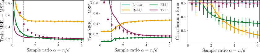
- Lower test loss does not mean better features:
- Linear autoencoders (PCA) always win on reconstruction loss (they rebuild the data best), but they completely miss the hidden factor.
- Nonlinear autoencoders have higher test loss—but they learn features that capture both hidden causes.
- On a simple downstream task (a small classification problem using the learned features), the nonlinear models perform much better.
- Practical warning:
- Using validation/test loss (like reconstruction error) to choose models or stop training can be misleading in self-supervised learning. A model with worse reconstruction may actually learn more useful features.
Why This Matters (Impact and Implications)
- For practice:
- Don’t rely only on reconstruction loss (or similar self-supervised test metrics) to judge feature quality.
- Evaluate with downstream tasks or linear probing to see if the model really captured useful structure.
- Choose activation functions wisely: some (like ReLU/ELU/Swish) can unlock hidden structure that linear methods miss.
- For theory:
- The paper provides a clean, solvable high-dimensional model that finally explains when and why tiny nonlinear networks beat PCA.
- It gives a concrete, testable example where “better test loss” does not mean “better generalization,” clarifying a common confusion in self-supervised learning.
A short analogy
- PCA is like using a straight ruler to find patterns—it’s great for straight-line relationships.
- Nonlinear autoencoders are like using a bendy ruler—they can follow curves and uncover patterns you can’t see with straight lines.
- This paper proves, in a simple world, that the bendy ruler can discover real structure the straight ruler misses—even if its drawings (reconstructions) look a bit less perfect.
Knowledge Gaps
Knowledge gaps, limitations, and open questions
Below is a concise list of unresolved issues and limitations that emerge from the paper. Each item is framed to be concrete and actionable for future research.
- Rigorous ERM theory beyond replica symmetry:
- The asymptotic characterization of empirical risk minimization (ERM) relies on the replica symmetric (RS) assumption. Provide a rigorous proof (or identify failure modes) by verifying the replicon condition and extending recent rigorous results to this model. Quantify whether RS holds across activations and sample ratios and derive consequences when RS breaks.
- Population dynamics beyond weak recovery:
- The gradient-flow analysis only covers early-stage dynamics up to weak recovery using low-order Hermite expansions. Develop a full dynamical analysis post–weak-recovery (fixed points, basins of attraction, convergence rates), either for specific latent distributions and activations or via general conditions on higher-order Hermite coefficients.
- Dependent latents with infinite correlation exponent:
- The case of dependent but uncorrelated latents with correlation exponent is left open. Determine whether any efficient algorithm (AMP or otherwise) can recover at , and characterize the statistical/computational thresholds under such dependence.
- AMP optimality and convergence guarantees:
- AMP is used as a proxy for efficient recovery and analyzed via linear stability at uninformed initialization. Prove (or refute) its optimality in this setting, establish global convergence conditions, characterize basins of attraction, and quantify sensitivity to initialization and damping.
- Explicit sample-complexity thresholds for nonlinear activations:
- Derive closed-form expressions for the weak recovery threshold as a function of latent distribution parameters and the first few Hermite coefficients of the effective nonlinearity. Compare thresholds across ReLU, ELU, Swish, GELU, Sigmoid, and custom activations.
- Spherical constraint vs unconstrained training:
- The population gradient-flow results assume a fixed radius . Analyze unconstrained training (as used in empirical ERM) with norm growth, weight decay, and normalization layers; characterize how radius (or norm dynamics) affects the key coefficients (, , ) and recovery.
- Non-smooth activations and approximation error:
- The theoretical analysis assumes smoothness (square-integrability) of the effective nonlinearity. Quantify how piecewise-linear/non-smooth activations (e.g., ReLU, GELU) can be accommodated without smoothing, and bound the approximation error when using smooth surrogates.
- Multi-unit and deeper autoencoders:
- Extend analysis from a single hidden unit with tied weights to multi-neuron, multi-layer, and untied-weight autoencoders. Determine minimal architectural requirements (width, depth, tying) to recover hidden spikes and how capacity affects and final overlaps.
- Competing nonlinear methods:
- Benchmark against other nonlinear representation learners (e.g., tensor methods, kernel PCA, ICA, score matching) that exploit higher-order moments. Identify which methods recover at comparable sample complexity and when autoencoders offer unique advantages.
- Strong recovery and asymptotic accuracy:
- The paper focuses on weak recovery (positive but small overlap). Characterize strong recovery (finite limiting overlap), derive conditions for asymptotically optimal overlap for both spikes, and quantify trade-offs between recovering vs .
- Finite-sample and finite-dimensional corrections:
- Systematically quantify deviations from asymptotic predictions at moderate . Provide finite-sample bounds on overlaps and losses, sensitivity to optimizer choice (GD vs Adam), learning rates, and stopping criteria.
- Misalignment of test loss and representation quality—generality:
- The misalignment is shown in this specific model. Identify necessary and sufficient conditions for such misalignment to occur in broader unsupervised/self-supervised settings and propose diagnostic metrics that detect when reconstruction/test loss is misleading.
- Downstream evaluation realism:
- The downstream task uses labels and a fixed linear predictor. Test robustness under realistic conditions: label noise, limited fine-tuning, non-linear probes, alternative tasks (e.g., clustering, regression), varying , and domain shift.
- Activation design principles:
- Translate the Hermite-coefficient conditions (, for small ) into actionable activation design guidelines. Search or learn custom activations that optimize recovery thresholds and downstream performance while controlling reconstruction loss.
- Early stopping and validation criteria:
- Develop principled early-stopping/selection rules that correlate with representation quality (e.g., higher-order moment probes, linear probing on small labeled sets, cumulant-based validation), and quantify failures of validation loss in guiding architecture and regularization choices.
- Role of whitening and model misspecification:
- The data-generating process uses whitening to hide from covariance. Assess robustness when whitening is imperfect/unknown to the learner or when latent variances are misspecified. Determine recovery conditions under model mismatch.
- More complex latent structure:
- Generalize to more than two spikes, multiple hidden factors with differing correlation exponents, structured dependence graphs among latents, and heavy-tailed/non-Gaussian latents. Analyze how these choices affect recoverability and thresholds.
- Untied weights in nonlinear autoencoders:
- For nonlinear AEs, tied weights may be suboptimal. Analyze whether untied encoder/decoder improves recovery of and/or lowers , and whether tying affects misalignment between loss and representation quality.
- Precise trade-off quantification:
- The paper observes that linear AEs recover at lower but miss . Quantify this trade-off analytically across activations, and characterize Pareto frontiers between reconstruction error and latent recovery.
- Robustness to noise and distributional shifts:
- Examine sensitivity to additive noise, outliers, non-Gaussian feature noise, and shifts in . Determine how these affect the Hermite spectrum, thresholds, and misalignment phenomena.
- RSB analysis for tanh and other cases:
- The mismatch for at small suggests possible RS breaking. Compute the replica symmetry breaking (RSB) solution (1RSB or full RSB) for the ERM objective with and identify the impact on predicted overlaps and losses.
- Computational-statistical gap assessment:
- The paper conjectures no statistical-to-computational gap based on AMP/BO agreement. Provide a formal assessment (lower bounds and algorithmic upper bounds) to confirm whether such gaps are absent or present, particularly for and in finite- regimes.
- Generalization of misalignment to other self-supervised objectives:
- Test whether similar misalignment arises under contrastive objectives, masked modeling, denoising autoencoders, or energy-based models. Identify objective designs that intentionally align with higher-order latent structure.
- Guidance for practical model selection:
- Turn the theoretical conditions into tools for practitioners: e.g., cumulant-based diagnostics to decide when to use nonlinear AEs; rules-of-thumb for activation choice; small-scale probes for hidden factor recoverability before full training.
Glossary
Below is an alphabetical list of advanced domain-specific terms from the paper, each with a concise definition and a verbatim usage example:
- Approximate-Message-Passing (AMP): A class of iterative algorithms for high-dimensional inference whose behavior can be tracked by deterministic “state evolution” and is often considered optimal among efficient methods. Example: "we introduce an Approximate-Message-Passing (AMP) algorithm for this problem."
- Baik-Ben Arous-Péché transition: A phase transition in random matrix theory where a signal spike causes an eigenvalue to detach from the bulk spectrum. Example: "it is the same as that of the Baik-Ben Arous-Péché transition \cite{baik2005phase} for the leading eigenvalue of the empirical covariance of the data"
- Bayes optimal (BO) estimator: The estimator given by the posterior average under a specified prior and data likelihood, achieving the best possible (information-theoretic) performance. Example: "The Bayes optimal (BO) estimator of the spikes is defined as "
- Correlation exponent: The smallest integer k such that the joint moment E[λk ν] is nonzero, indicating the first order at which latent dependence appears beyond linear correlation. Example: "We define the correlation exponent of a distribution as the smallest such that ."
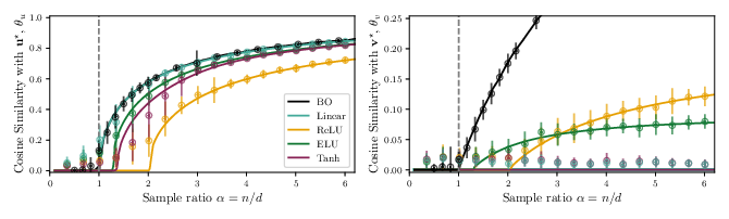
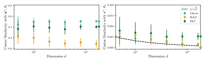
- Cosine similarity: A normalized inner product that measures the alignment between two vectors (magnitude-invariant). Example: "Additionally, the cosine similarities concentrate to"
- Downstream task: A supervised task used to evaluate representations learned in an unsupervised or self-supervised stage. Example: "we introduce a simple downstream task that allows principled evaluation without direct access to the ground-truth spikes."
- Eckart--Young theorem: A theorem stating that PCA provides the optimal low-rank approximation in squared error (Frobenius norm). Example: "linear autoencoders are equivalent to PCA and are optimal for squared reconstruction error by the Eckart--Young theorem \cite{eckart1936approximation}."
- ELU: An activation function (Exponential Linear Unit) that is smooth and can aid learning in nonlinear autoencoders. Example: "Non-linear autoencoders with other considered activations (Relu, ELU, but also Swish, Sigmoid and GELU see \cref{app:k2_activations_GD})"
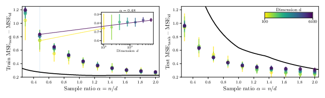
- Empirical risk minimization (ERM): The principle of minimizing average loss over a finite dataset to learn model parameters. Example: "We study the global minimum of the empirical risk \cref{eq:empiricalrisk} along similar technical lines to \cite{cui2023high}."
- Frobenius norm: A matrix norm equal to the square root of the sum of squared entries, commonly used to measure approximation error. Example: "equivalently the best rank-one approximation in Frobenius norm \cite{eckart1936approximation}."
- GELU: An activation function (Gaussian Error Linear Unit) that provides smooth nonlinear transformations in neural networks. Example: "but also Swish, Sigmoid and GELU see \cref{app:k2_activations_GD}"
- Hermite polynomials: Orthogonal polynomials under the Gaussian measure used to expand functions in high-dimensional probabilistic analysis. Example: "probabilists' Hermite polynomials are denoted with $\He_k$"
- High-dimensional limit: An asymptotic regime where both dimension and sample size grow (often proportionally), enabling tractable analyses. Example: "in the high-dimensional limit with ."
- Information-theoretically optimal estimator: An estimator that achieves the best possible performance allowed by the statistical structure of the problem, irrespective of computational constraints. Example: "gives the performance of the information-theoretically optimal estimator for the spikes"
- Leading eigenvector: The eigenvector associated with the largest eigenvalue of a matrix; in PCA, the principal component direction. Example: "and is a leading eigenvector of the covariance ."
- Likelihood ratio: The ratio of the data-generating density to a reference density, used to reweight expectations under a convenient distribution. Example: "in which we introduced the likelihood ratio "
- Linear probing: A protocol where a linear classifier is trained on top of learned representations to evaluate their usefulness. Example: "it is evaluated almost exclusively via downstream tasks or linear probing \cite{grill2020bootstrap, he2022masked, devlin2019bert, balestriero2024learning}."
- Order parameters: Low-dimensional summary quantities (e.g., overlaps) that characterize the macroscopic state of a learning system. Example: "Define the order parameters"
- Outlying eigenvalue: An eigenvalue that separates from the bulk spectrum due to signal, indicating detectability of a spike. Example: "only for the covariance \cref{eq:cov-intro} develops an outlying eigenvalue, with eigenvector correlated with ."
- Population risk: The expected loss computed with respect to the true data-generating distribution, rather than a finite sample. Example: "At the population level, the objective reads"
- Posterior average: The expectation under the posterior distribution; in Bayes estimation, it yields the optimal estimator under squared loss. Example: "such BO estimator is given by the posterior average, i.e. the mean of the probability distribution"
- Prior (distribution): The probability distribution over parameters before observing data, used in Bayesian inference. Example: "where we denoted by the distribution of the spikes (isotropic Gaussian in our case)"
- Relu: An activation function (Rectified Linear Unit) defined as max(0, x), widely used in deep learning. Example: "Non-linear autoencoders with other considered activations (Relu, ELU, but also Swish, Sigmoid and GELU see \cref{app:k2_activations_GD})"
- Replica method: A technique from statistical physics for analyzing complex random systems via replicated variables; often used to derive asymptotic characterizations. Example: "\cref{res:bo} is derived in \cref{app:BO_AMP} using the replica method from statistical physics."
- Replica symmetric assumption: An assumption that all replicas behave identically, simplifying replica-based analyses. Example: "under the so-called replica symmetric assumption (see \cref{app:replica_computation}) the order parameters concentrate onto their mean"
- Replicon condition: A stability condition in replica theory ensuring the validity of the replica symmetric solution. Example: "and to show that the so-called replicon condition described therein holds."
- Self-supervised learning: Learning representations from unlabeled data using auxiliary tasks or constraints, without ground-truth labels. Example: "In modern self-supervised learning, representation quality is rarely assessed through reconstruction or test loss"
- Sigmoid: A logistic activation function mapping real numbers to (0, 1), used in neural networks. Example: "but also Swish, Sigmoid and GELU see \cref{app:k2_activations_GD}"
- Single index model: A model where the response depends on data only through a single linear projection passed through a nonlinearity. Example: "using recent advances for the supervised learning of the single index model using stochastic gradient descent"
- Spherical constraint: A constraint enforcing that a parameter vector lies on a sphere (fixed norm), used to regularize dynamics. Example: "subject to a spherical constraint on ."
- Spherical gradient flow: Gradient descent dynamics projected onto the sphere manifold, maintaining the spherical constraint. Example: "Consider spherical gradient flow dynamics on the population loss, i.e. the following dynamical system:"
- Spiked covariance model: A random data model with a low-rank signal added to an identity covariance, used to study high-dimensional inference limits. Example: "the spiked covariance model and its variants \cite{baik2005phase,johnstone2009consistency,donoho2018optimal,deshpande2014information,lelarge2017fundamental}"
- Spiked cumulant model: A data model where latent structure is encoded in higher-order moments (cumulants), potentially invisible to covariance. Example: "who introduced the spiked cumulant model in which a dataset of samples in dimension is generated as"
- State evolution: A deterministic recursion describing the dynamics of AMP in the high-dimensional limit. Example: "the so-called state evolution, see for e.g. \cite{bayati2011dynamics,berthier2020state}"
- Swish: A smooth activation function defined as x·sigmoid(x), used to improve nonlinear representation learning. Example: "but also Swish, Sigmoid and GELU see \cref{app:k2_activations_GD}"
- tanh: The hyperbolic tangent activation function mapping inputs to (-1, 1), used in neural networks. Example: "For the activation and correlation exponent "
- Weak recovery: Attaining nonzero correlation with true latent directions in the high-dimensional limit (not necessarily exact reconstruction). Example: "Characterization of the weak recovery of ."
- Whitening matrix: A linear transformation that normalizes and decorrelates components, making certain directions invisible to covariance. Example: "is a whitening matrix."
Practical Applications
Summary
This paper introduces a tractable high-dimensional “spiked cumulant” data model where:
- Nonlinear autoencoders (even a 1-unit, tied-weights AE) provably recover latent structure that is invisible to PCA and linear AEs.
- The “hidden” latent factor is uncorrelated with observable features at second order but present in higher-order moments; recovery depends on finite correlation exponent k* (smallest k with E[λk ν] ≠ 0).
- Certain activations (e.g., ReLU, ELU, Swish, Sigmoid, GELU) enable recovery at k*=2 with O(d log d) samples, while tanh may fail at k*=2 but succeed at k*=3.
- Self-supervised test reconstruction loss can be misaligned with representation quality: linear AEs achieve lower loss yet fail to recover meaningful latent structure; nonlinear AEs recover it despite higher loss.
- The work provides analytical tools (population risk, ERM via replica methods, AMP baselines), a clear benchmark model, and actionable diagnostics for SSL evaluation.
Below are practical applications and workflows derived from these findings.
Immediate Applications
- Software/ML engineering (self-supervised learning pipelines)
- Replace “validation/test reconstruction loss” as the sole model-selection criterion with downstream linear-probe or small-label tasks that explicitly test for latent recovery.
- Introduce early-stopping guardrails based on representation quality (e.g., linear-probe accuracy plateau) rather than minimal validation loss.
- Tools/products: “Representation Alignment Dashboard” that tracks test loss vs. downstream probe metrics and flags misalignment; lightweight linear-probe evaluation harness integrated into training loops.
- Assumptions/dependencies: downstream tasks must be chosen to reflect latent structure of interest; modest labeled subset available; compute budget for probes.
- Data science practice (daily life of analysts)
- When PCA finds no signal, try a minimal 1-neuron nonlinear autoencoder (with ReLU/ELU/Swish/GELU/Sigmoid) to capture higher-order dependencies.
- Workflow: standardize/whiten features → train small nonlinear AE → evaluate features with a simple linear classifier on a tiny labeled subset.
- Assumptions/dependencies: sufficient sample ratio n/d (ideally O(d log d) for rapid weak recovery); activation choice matters (avoid tanh for k*=2 scenarios).
- Model/activation selection guidelines
- Prefer non-saturating activations (ReLU/ELU/Swish/GELU) for data where structure is suspected beyond covariance; avoid tanh for low-order (k*=2) higher-moment structure.
- Tools/products: “Activation Selector” that recommends activations by inspecting low-order Hermite interactions or proxies of higher-order dependence in the dataset.
- Assumptions/dependencies: ability to estimate simple statistics (e.g., proxies for E[λk ν]); performance depends on data scaling/whitening.
- Benchmarking and reproducible research (academia and industry R&D)
- Use the spiked cumulant model as a minimal, controllable benchmark where nonlinear methods provably beat PCA and test loss can mislead selection.
- Tools/products: Benchmark generator (based on the authors’ code) with configurable k*, sample ratio α=n/d, and activation sweeps to test SSL algorithms.
- Assumptions/dependencies: synthetic model approximates real data regimes with higher-order dependencies; reproducibility relies on provided code.
- Risk management and governance for SSL (policy and enterprise ML governance)
- Update internal evaluation policies to require downstream/linear-probe reporting alongside validation loss for SSL or generative pretraining.
- Introduce “misalignment checks” in model cards: document cases where lower reconstruction loss degraded downstream performance.
- Assumptions/dependencies: availability of appropriate proxy tasks; stakeholder buy-in to shift evaluation culture beyond loss-only metrics.
- Sector-focused pilots
- Healthcare (EHR, omics), Finance (returns, limit-order books), Cybersecurity (network telemetry), IoT/Industry 4.0 (multisensor time series):
- Deploy small nonlinear AEs as a feature discovery stage where PCA finds little; validate via micro-tasks (anomaly flags, short-horizon predictions).
- Tools/products: “Higher-Order Feature Extractor” module dropped into existing data pipelines; quick linear-probe validators for anomaly/label-lite tasks.
- Assumptions/dependencies: enough samples (relative to feature dimension), careful standardization; formal guarantees hold in high-dimensional regime.
- MLOps instrumentation
- Add metrics capturing representation quality (linear-probe accuracy, clustering separability) to training dashboards; correlate or de-correlate them from test loss.
- Tools/products: Plugins for MLFlow/Weights & Biases that compute and track probe metrics and “loss–representation misalignment” indicators.
- Assumptions/dependencies: small labeled slices available; additional compute for periodic probes.
- Education and training
- Demonstrate PCA limitations vs. nonlinear AE capabilities using the paper’s code in course labs; show test-loss vs. representation misalignment concretely.
- Assumptions/dependencies: students can run small synthetic experiments; access to the provided GitHub repository.
Long-Term Applications
- Next-generation SSL objectives targeting higher-order structure (software/ML research)
- Design pretext losses or regularizers that directly exploit higher-order cumulants (e.g., moment-matching beyond covariance) for improved latent recovery.
- Products/workflows: “Higher-Order SSL” libraries that augment contrastive/masked modeling with cumulant-aware terms; automated moment-adaptive training.
- Assumptions/dependencies: scalable estimators of higher moments; robustness to real-data deviations from the model.
- Automated estimation of correlation exponent and sample complexity
- Build robust estimators or model selection criteria that infer effective k* (or proxies) to guide activation choice, architecture depth, and sample needs.
- Products: “k*-Estimator” service; “Sample Complexity Advisor” that recommends data collection targets (n) to cross weak-recovery thresholds.
- Assumptions/dependencies: reliable higher-moment estimation under finite samples; robust to heteroskedasticity and outliers.
- AMP-inspired algorithms and tooling for unsupervised recovery
- Adapt and harden Approximate Message Passing for real-world data to approach Bayes-optimal recovery when higher-order dependencies exist.
- Products: “AMP-Pretrainer” that initializes or complements AEs; hybrid AMP+GD routines.
- Assumptions/dependencies: algorithmic stability beyond idealized Gaussian settings; engineering for large-scale, non-i.i.d. data.
- Domain-specific systems exploiting higher-order latent recovery
- Healthcare/genomics: representation learners that uncover interaction effects (epistasis, pathways) invisible to covariance for diagnosis or discovery.
- Finance: factor models capturing nonlinear risk components for stress testing and portfolio construction.
- Cybersecurity/IoT/energy grids: anomaly detectors sensitive to coordinated but covariance-invisible events; predictive maintenance with early-warning signals.
- Products: verticalized “Higher-Order Representation” modules integrated into EHR analytics, risk engines, SOC pipelines, and SCADA monitoring.
- Assumptions/dependencies: regulatory compliance (e.g., medical devices), rigorous validation on real datasets; careful handling of distribution shift.
- Robust evaluation standards and regulation for SSL
- Establish industry standards that discourage over-reliance on validation loss, requiring representation-quality benchmarks (linear probe suites, task batteries).
- Policy artifacts: guidance documents, procurement checklists, and compliance tests for foundation/self-supervised models.
- Assumptions/dependencies: consensus on proxy tasks; availability of public benchmark suites; collaboration between regulators and standards bodies.
- Architecture design with provable properties
- Develop shallow nonlinear AEs or simple multi-unit architectures with guarantees of weak recovery under broad data conditions; extend to multi-spike, multimodal settings.
- Products: “Provable AE” blueprints for edge or embedded inference where simplicity and assurances matter (e.g., industrial inspection).
- Assumptions/dependencies: theory extensions beyond single-unit, tied weights; real-data validation.
- Fairness and bias diagnostics via hidden-factor recovery
- Use higher-order-sensitive representations to reveal latent subgroup structure that PCA misses; support fairness audits and bias mitigation.
- Products: “Latent Subgroup Auditor” that probes for hidden factors affecting downstream disparities.
- Assumptions/dependencies: ethical data use, governance approvals; careful interpretation to avoid spurious subgrouping.
- Lightweight edge analytics
- Embed minimal nonlinear AE feature extractors on-device (sensors, wearables) to detect subtle, coordinated changes with tiny footprint.
- Products: firmware modules for microcontrollers; streaming anomaly flags sent upstream for consolidation.
- Assumptions/dependencies: offline training or federated updates; resource constraints; privacy constraints.
- Curriculum and workforce upskilling
- Incorporate higher-order dependence concepts, activation impacts, and loss–generalization misalignment into ML curricula and professional development.
- Assumptions/dependencies: accessible teaching materials; open-source toolkits and labs.
Cross-Cutting Assumptions and Dependencies
- High-dimensional regime and model match: Results are strongest when data resemble the spiked cumulant model (two latent factors, one only visible via higher moments) and d is large.
- Finite correlation exponent k*: Recovery hinges on existence of some k with E[λk ν] ≠ 0; if k* = ∞ or latents are independent, recovery may require many more samples or be infeasible with simple methods.
- Sample complexity: For weak recovery in practice, aim for α = n/d at or above O(1), with O(d log d) samples for fast dynamics under favorable activations.
- Activation choice: Non-saturating activations (ReLU/ELU/Swish/GELU/Sigmoid) enable recovery for k*=2; tanh may require k*≥3 or more samples.
- Scaling/whitening and constraints: Whitening and appropriate weight scaling (spherical norm analogs) can affect learnability; mismatches may degrade outcomes.
- ERM analysis relies on replica-symmetric assumptions; deviations in some regimes (e.g., tanh at small α) may occur.
- Misalignment caveat: Lower reconstruction loss does not guarantee better representations; pipelines must incorporate downstream or probing metrics to avoid misguided selections.
These applications can be enacted incrementally: start with diagnostic benchmarking and activation-aware AE baselines plus downstream probes, then evolve toward higher-order-aware SSL objectives, robust k* estimation, and sector-specific deployments.
Collections
Sign up for free to add this paper to one or more collections.

