Solar and anthropogenic climate drivers: an updated regression model and refined forecast
Abstract: In a paper attempts were made to quantify the respective solar and anthropogenic influences on the terrestrial climate, and to cautiously predict the global mean temperature over the next 130 years. In a double regression analysis, both the binary logarithm of carbon dioxide concentration and the geomagnetic aa-index were used as predictors of the sea surface temperature (SST) since the mid-19th century. The regression results turned out to be sensitive to end effects, leading to a broad range of the climate sensitivity between 0.6 K and 1.6 K per doubling of CO$_2$ when varying the final year. The aim of this paper is to narrow down this range. To this end, the correlations between the two predictors and the dependent variable (SST) are analysed in detail. It is demonstrated that the SST can be predicted until around 2000 almost perfectly using only the aa-index, whereas for later periods the role of CO$_2$ increases significantly. Hence, the weight of the aa-index is fixed to its robust outcome (around 0.04 K/nT) from the regressions up to 1990. The SST data, reduced by the aa-contribution thus specified, are then used in a single regression with CO$_2$ as the only remaining predictor. This results in a significant reduction in the range of CO$_2$ sensitivity, narrowing it to 1.1-1.4 K. Given the exceptionally high temperatures in recent years, these values are considered a kind of upper limit that could still be subject to downward corrections when future data are incorporated. Based on this estimate, the temperature forecast until 2100 is refined by using more precise predictions of the aa-index and the paths of atmospheric CO$_2$ content which are based on constant emission scenarios combined with a linear sink model. With the exception of the most ``pessimistic'' variant, the temperature is predicted to remain below the extraordinarily high value measured in 2024.
Paper Prompts
Sign up for free to create and run prompts on this paper using GPT-5.
Top Community Prompts
Explain it Like I'm 14
Overview: What this paper is about
This paper looks at two main things that can affect Earth’s temperature:
- Changes linked to the Sun
- Greenhouse gases made by humans, especially carbon dioxide (CO2)
The author tries to figure out how much each of these has influenced global sea surface temperatures since the mid-1800s and then uses that to make a simple temperature forecast up to the year 2100.
The big questions the paper asks
- How much of the warming in the last 170+ years can be explained by solar activity, and how much by CO2?
- Can we get a tighter (more precise) estimate of “climate sensitivity”—how much the global temperature rises when CO2 doubles?
- Based on those estimates, what might global temperatures look like by 2100?
How the study was done (in simple terms)
Think of predicting temperature like baking a cake with two main ingredients:
- A “solar activity” ingredient
- A “CO2” ingredient
The author uses a math method called “regression” (a way to fit a line to data) to decide how much each ingredient contributes to the final “cake” (sea surface temperature). Here’s how it works:
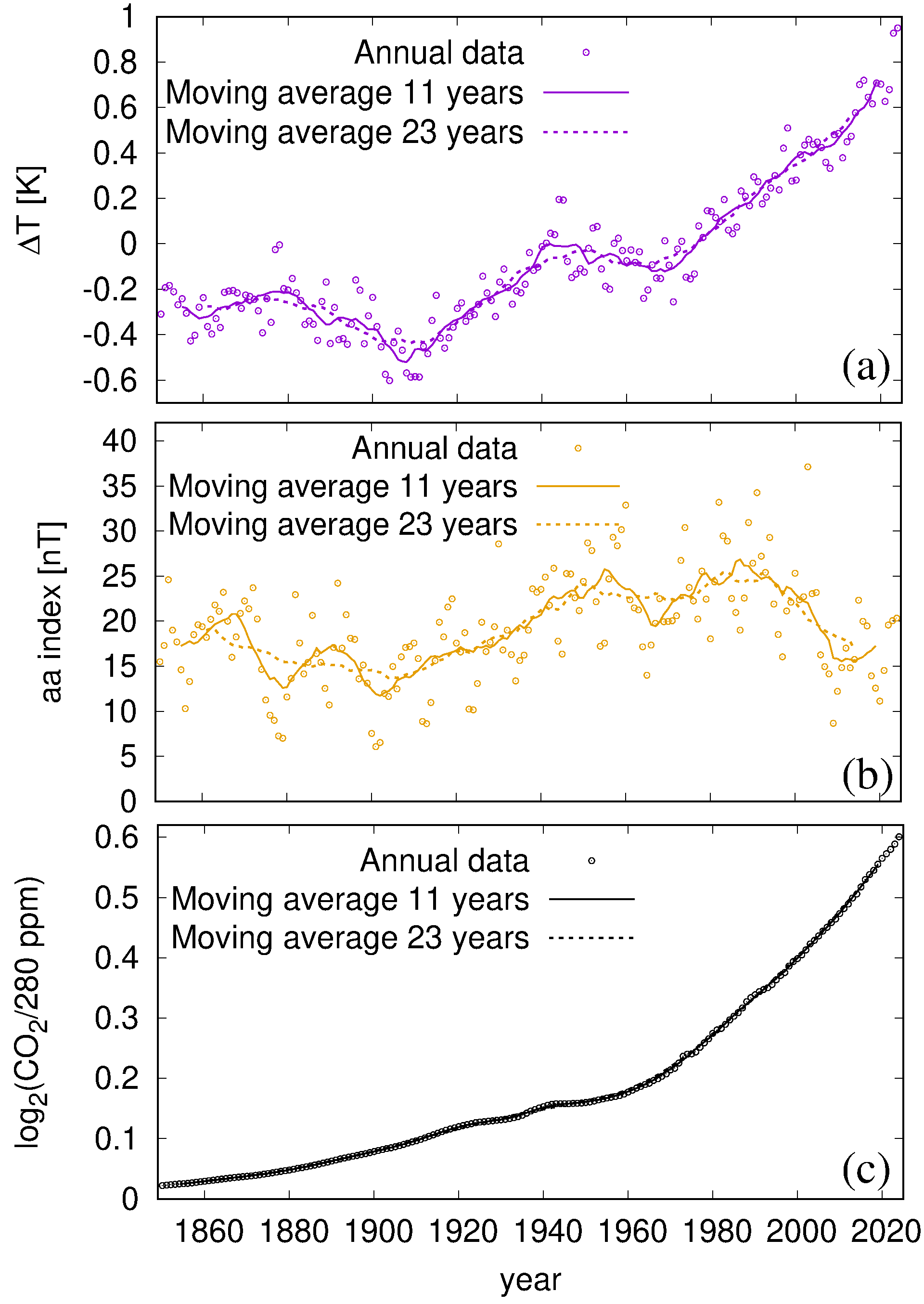
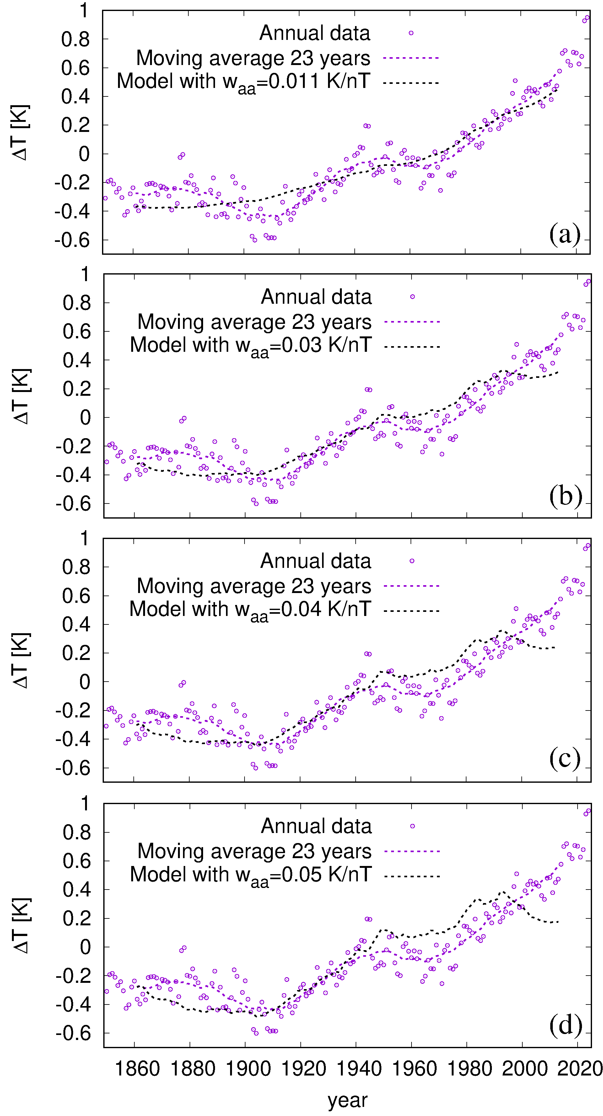
- Temperature data: Global sea surface temperature changes from 1850–2024 (relative to the average from 1961–1990).
- Sun data: A number called the “aa-index,” which measures how much the Sun’s activity stirs up Earth’s magnetic field. It’s used here as a simple “proxy” (stand-in) for overall solar influence.
- CO2 data: The author uses the binary logarithm of CO2, written as log2(CO2/280 ppm). This just means “how many times has CO2 doubled since preindustrial times (about 280 ppm)?” For example, a doubling corresponds to 1 on this scale.
To make the trends clearer, the author smooths the data using moving averages over 11 or 23 years. You can think of this like blurring a picture slightly so you can better see the main shapes without being distracted by small wiggles.
A key challenge is that the aa-index and CO2 both tend to rise and fall over long timescales, which makes them partly “collinear.” In everyday language: when two ingredients rise together, it’s hard to know how much each one really matters. That can make the results overly sensitive to what years you include at the end of the record.
To deal with that, the author:
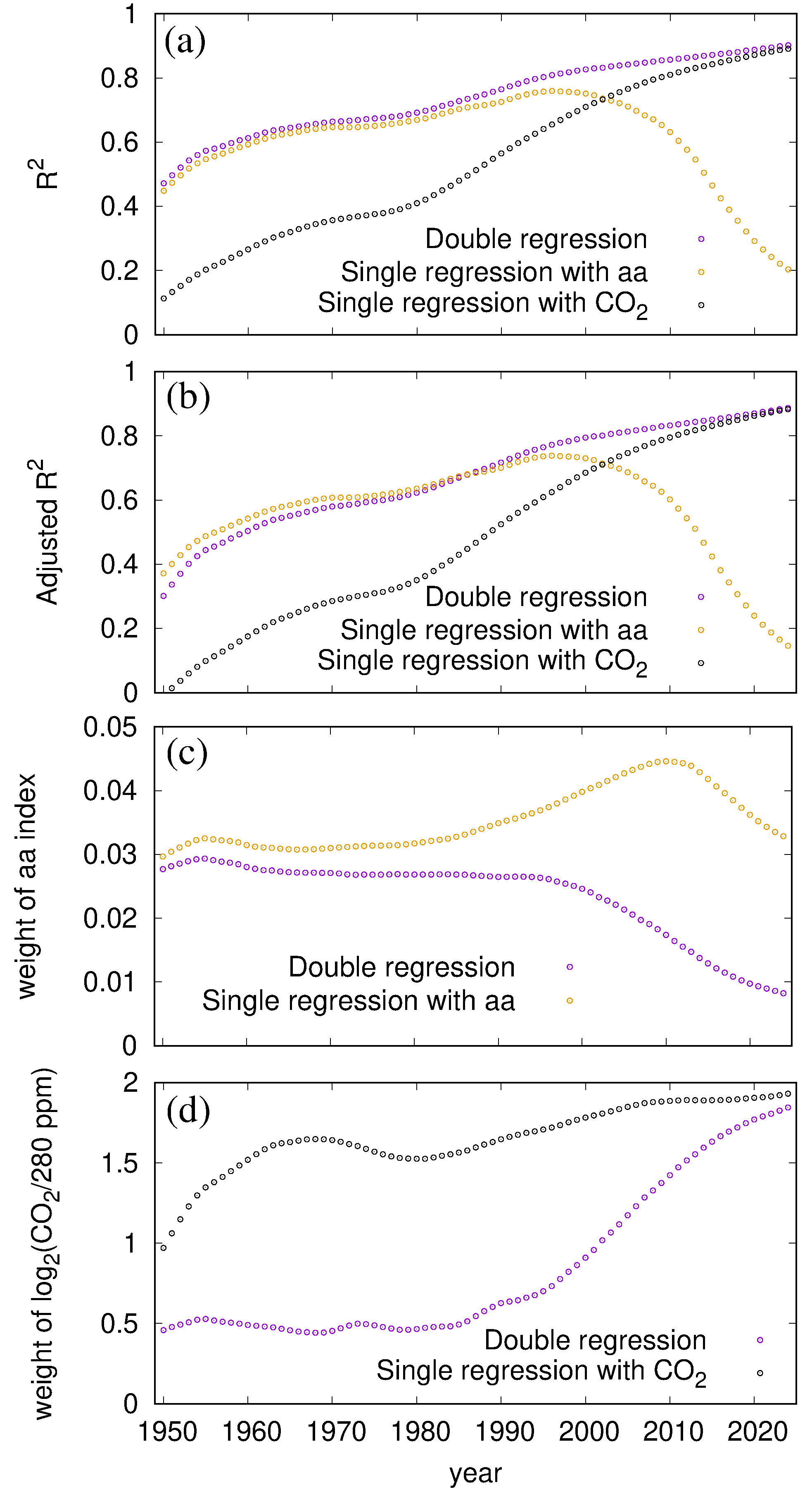
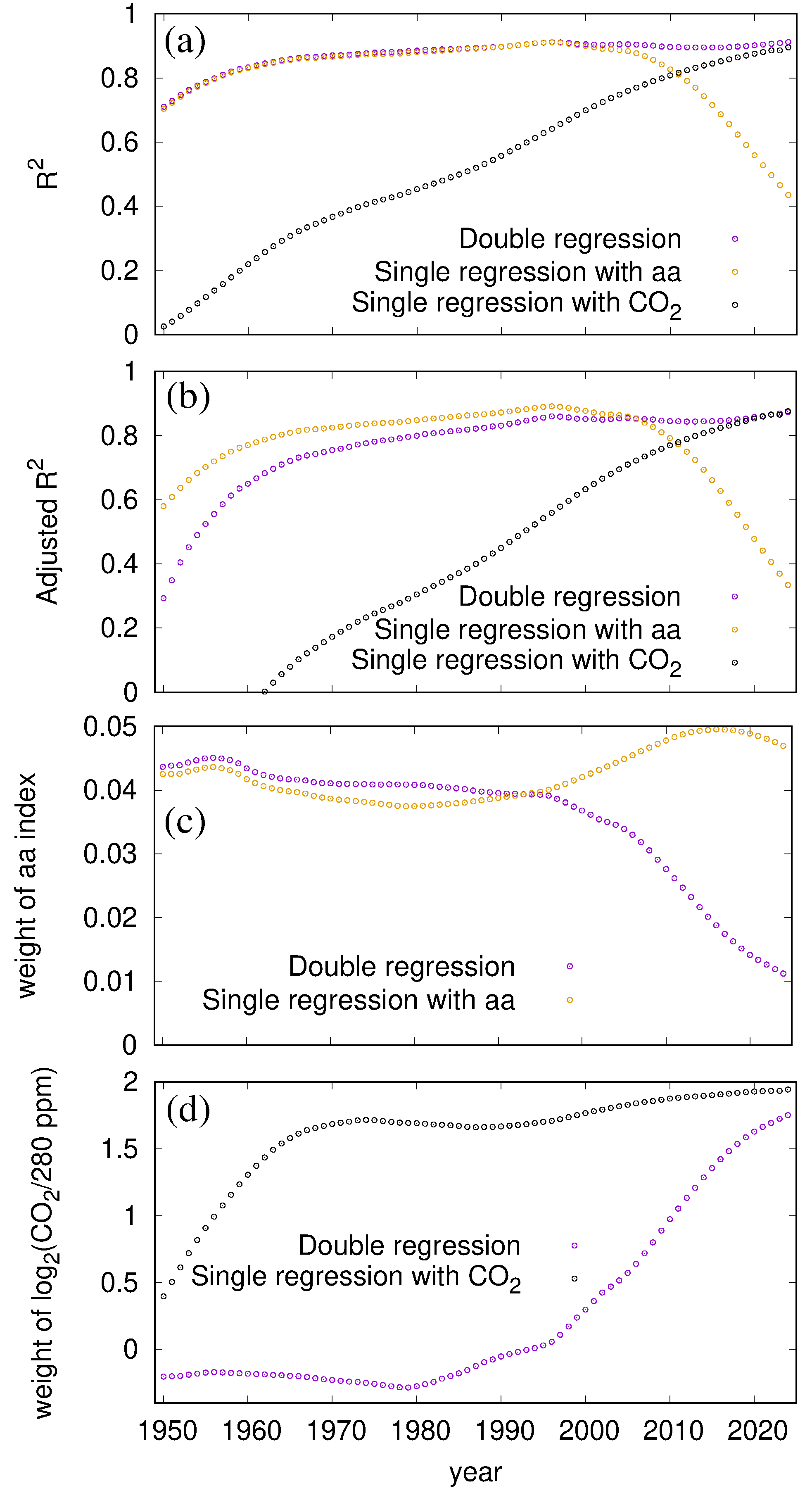
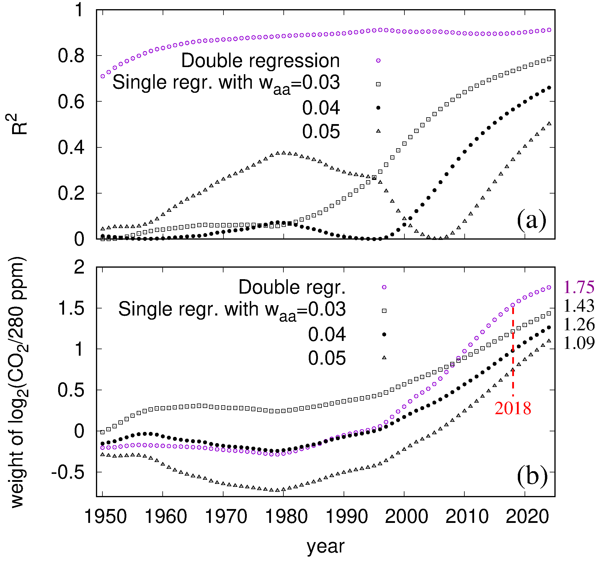
- First checks how well each ingredient works on its own.
- Notices that until about the late 1990s–early 2000s, the Sun’s aa-index alone matches sea surface temperatures surprisingly well.
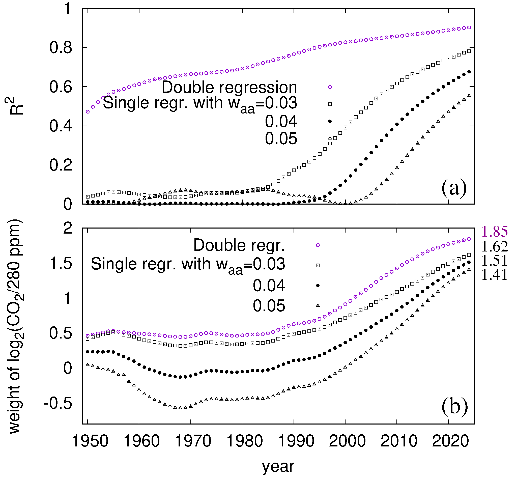
- Fixes (locks in) the Sun’s “weight” at a stable value found from the earlier period (about 0.04 K per nT, where K is degrees Celsius and nT is the unit for the aa-index).
- Subtracts the Sun’s contribution from the temperature record.
- Then runs a simple one-ingredient regression using only the remaining temperature and CO2. This aims to give a steadier estimate of how sensitive temperature is to CO2, without the two ingredients “fighting” each other in the math.
Finally, to make a forecast to 2100, the paper:
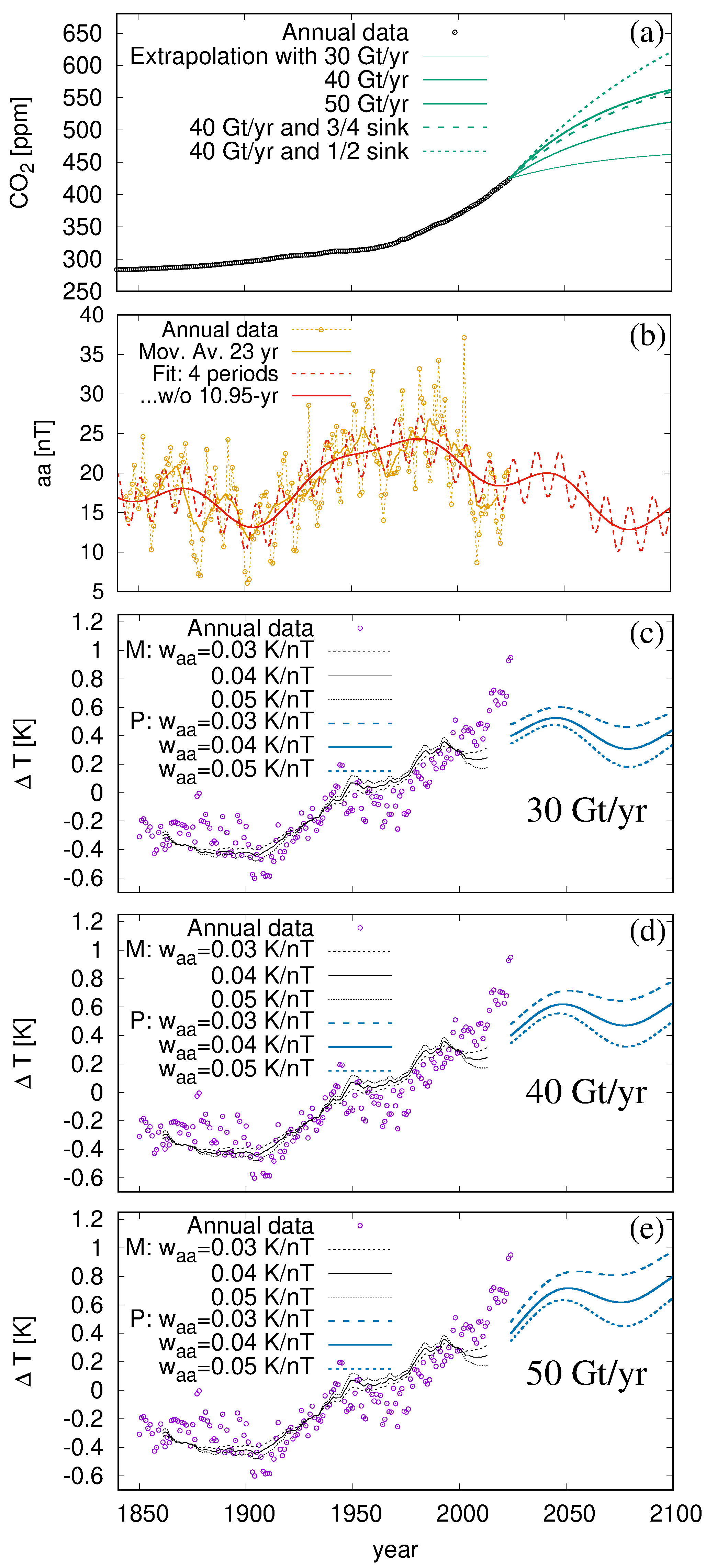
- Predicts future CO2 using simple scenarios of constant yearly emissions (30, 40, or 50 billion tons of CO2 per year) and a “linear sink” model. The sink model assumes Earth (oceans and plants) absorbs more CO2 when the air has more above preindustrial levels, in a way that’s roughly proportional.
- Predicts the Sun’s future ups and downs using a solar cycle model with a few repeating periods (approximately 11, 57, 90, and 193 years), then converts that into a future aa-index.
- Combines the Sun part and the CO2 part to get a temperature forecast.
Main findings and why they matter
Here is what the study says, in plain language:
- Up to around 2000, temperature changes can be explained very well using the Sun’s aa-index alone. After 2000, CO2 becomes more important.
- When the aa-index “weight” is fixed at a steady value that fits the earlier data (about 0.04 K per nT), the remaining CO2 effect comes out to a climate sensitivity of about 1.1–1.4 K of warming for each doubling of CO2. The paper treats this as closer to a “Transient Climate Response” (TCR), which is a medium-term warming measure.
- Using the author’s preferred settings, the forecast suggests that by 2100 the global temperature (compared to the 1961–1990 average) might be about 0.6 K higher in the “middle” emissions case, with a spread of roughly ±0.3 K depending on the chosen solar and CO2 settings and whether emissions are 30, 40, or 50 billion tons per year.
- In most of the forecast versions, temperatures by 2100 stay below the very high value measured in 2024, except in the most pessimistic case (high emissions, higher CO2 sensitivity, lower solar influence).
Why this matters: If these results are correct, CO2’s medium-term warming effect could be at the lower end of other recent estimates, and solar changes could play a bigger role than many models assume—especially for earlier decades. That would imply a more modest amount of warming by 2100 under constant emissions.
Implications, limits, and what to watch next
What this could mean:
- If the paper’s approach is right, medium-term warming from CO2 might be smaller than many other studies suggest, and natural solar variations could be a larger driver than often modeled.
- The forecast suggests a relatively “benign” rise by 2100 in the scenarios tested, with most cases staying under 1 K above the 1961–1990 average.
Important limitations to keep in mind:
- The study deliberately leaves out some short-term drivers like El Niño and large volcanic effects, which can strongly affect temperatures in certain years.
- It uses the aa-index as a proxy for the Sun’s climate influence and a solar cycle model to predict future aa-index; both choices come with uncertainties.
- The “fix-then-regress” step (fixing the Sun’s weight and then estimating CO2’s effect) is a nonstandard strategy used to avoid a math problem called collinearity. It’s a reasonable idea to test, but it’s still a judgment call.
- Future CO2 emissions, and how the Earth absorbs CO2, may change in ways this simple model doesn’t capture.
What to watch:
- How temperatures behave in the next few years (do they stay unusually high or ease back?).
- New data on solar activity and better measurements of how Earth absorbs CO2.
- Studies that include more factors (like El Niño and volcanoes) to see whether the main conclusions hold up.
In short: This paper argues that the Sun explained much of the earlier warming, CO2 has become more important in recent decades, and that CO2’s medium-term warming effect may be on the lower side of other estimates. If that’s true, the future warming in the tested scenarios would likely be moderate. But the results depend on specific modeling choices and assumptions, so more data and comparisons with other methods will be important.
Knowledge Gaps
Unresolved gaps, limitations, and open questions
The following list identifies what remains missing, uncertain, or unexplored in the paper, formulated to guide concrete future research steps.
- Quantify and model the physical mechanism linking the geomagnetic aa-index to SST (e.g., via stratospheric–tropospheric coupling, UV–ozone pathways, solar wind–electrical circuit impacts, or cosmic ray–cloud interactions), including expected sign, lags, and regional fingerprints.
- Test whether the inferred aa sensitivity (~0.03–0.05 K/nT) is time-invariant or state-dependent by estimating time-varying coefficients (e.g., state-space/Kalman models) and examining regime shifts in circulation (Hadley widening, storm track shifts).
- Address multicollinearity between aa and CO2 rigorously using methods such as cointegration/error-correction models, instrumental variables, ridge/LASSO regularization, or partial regression to disentangle trend-dominated predictors.
- Explicitly model and test time lags between predictors (aa, CO2) and SST (cross-correlation, distributed-lag or transfer-function models) to avoid bias from synchronous regression on smoothed series.
- Include major confounders (ENSO, volcanic aerosols including Hunga Tonga–Hunga Ha’apai, anthropogenic aerosol forcing, AMO/PDO) as covariates and quantify their effect sizes; test if their inclusion stabilizes w_aa and w_CO2 estimates.
- Evaluate robustness to the choice of temperature dataset by repeating analyses with alternative SST products (ERSSTv5/6, HadISST) and global surface temperature datasets (e.g., HadCRUT, Berkeley Earth), including quantified data uncertainties and potential measurement biases.
- Provide formal uncertainty quantification for w_aa and w_CO2 (confidence/credible intervals), accounting for autocorrelation, smoothing-induced degrees-of-freedom loss, and end-point effects; validate the adjusted R² calculation for smoothed series.
- Test for spurious correlation due to common trends by detrending/decomposing series (e.g., differencing, STL decomposition) and reassessing relationships on variability components rather than long-term trends alone.
- Perform out-of-sample validation (e.g., rolling-origin forecasts, withheld decades) to assess predictive skill of aa-only and aa+CO2 models over distinct historical intervals.
- Compare the regression-based TCR estimates against physically constrained energy-balance models (one-/two-box EBMs) that incorporate ocean heat uptake and thermal inertia; reconcile differences and identify conditions under which each approach is valid.
- Expand greenhouse forcing beyond CO2 to include CH4, N2O, halocarbons, tropospheric ozone, and land-use albedo changes to avoid attributing their warming to either aa or CO2 implicitly.
- Investigate whether the early 20th-century warming (1905–1940) attributed to aa can instead be explained by internal variability (AMO) and aerosols; apply attribution methods (optimal fingerprinting) to separate forcings and modes.
- Assess sensitivity of results to smoothing choices (MAW length, centered vs trailing windows, LOESS/Butterworth filters) and to endpoint handling, demonstrating that conclusions are robust across preprocessing methods.
- Examine residual structure (autocorrelation, heteroskedasticity, nonstationarity) and apply appropriate time-series methods (ARIMAX, GLS) rather than OLS on smoothed data to ensure valid inference.
- Provide and validate a causal inference framework (e.g., Granger causality tests, structural causal models) to distinguish correlation from causation in aa–temperature and CO2–temperature relationships.
- Quantify and propagate uncertainties from the synchronized solar dynamo aa forecast (periods, amplitudes, phases), and compare its predictive skill to alternative solar activity reconstructions (TSI composites, F10.7, Ap/AE indices).
- Test the assumption of fixed dominant solar periods (193, 90, 57 years, Schwabe ~10.95 years) against observational variability; evaluate how deviations in phase/amplitude alter temperature forecasts.
- Improve carbon-cycle modeling beyond a linear sink with constant B by incorporating temperature-dependent sinks, saturation/nonlinearity, land–ocean partitioning, and policy/land-use dynamics; estimate B(t) with uncertainty ranges and scenario dependence.
- Provide probabilistic temperature projections (with uncertainty bands) by propagating uncertainties in aa forecasts, carbon sinks/emissions, and sensitivity parameters, rather than deterministic trajectories.
- Benchmark forecasts against CMIP6/AR6 scenarios and observational constraints (e.g., CERES TOA fluxes, ocean heat content), identifying where and why the paper’s projections diverge.
- Explore regional impacts and mechanisms (e.g., North Atlantic circulation, cyclone tracks) to test whether aa-linked top-down pathways produce distinctive spatial patterns consistent with observations.
- Document full reproducibility (code, parameter choices, preprocessing steps), enabling independent replication and sensitivity analyses by other researchers.
- Clarify the treatment of SST vs global mean surface temperature: assess whether conclusions hold when land temperatures are included and when using a globally complete metric for climate sensitivity and policy relevance.
- Resolve the contribution of the 2023–2024 temperature spike by quantitatively attributing shares to ENSO, stratospheric water vapor from Hunga Tonga, anthropogenic aerosols, and greenhouse gases, and testing the impact on inferred w_CO2 and w_aa.
- Determine whether the aa sensitivity decline seen in late double regressions reflects real physical changes or model misspecification; design tests to discriminate these possibilities (e.g., adding missing forcings, allowing time-varying coefficients).
- Assess long-term boundary conditions (Milanković cycles, potential grand solar minima) within a framework that separates transient (TCR-like) responses from equilibrium (ECS) to avoid conflating multi-century drivers with 21st-century projections.
Practical Applications
Overview
This paper proposes a two-stage regression framework that separates solar-activity-driven variability (proxied by the geomagnetic aa-index) from CO2-driven warming to narrow the range of transient climate sensitivity (TCR-like) to CO2 doubling to about 1.1–1.4 K. It also offers a simplified forecasting workflow that combines:
- A fixed aa-index sensitivity estimated from pre-1990 data, then subtracted from SST anomalies.
- A single regression on CO2 for the residuals.
- A synchronized solar dynamo model (with fixed 193, 90, 57-year periods plus a 10.95-year component) to forecast the aa-index.
- A linear carbon sink model with constant-emissions scenarios (30, 40, 50 Gt CO2/yr) to forecast atmospheric CO2.
Below are practical applications derived from the paper’s methods and results. Each item notes sectors, potential tools/products/workflows, and key assumptions/dependencies.
Immediate Applications
These can be piloted or deployed now, using existing data and modeling capabilities, while acknowledging uncertainties and the need for validation.
- Climate sensitivity estimation toolkit using two-stage regression
- Sectors: academia, climate services, finance (risk), policy analysis.
- Tool/product/workflow: open-source package that (i) ingests HadSST, aa-index, and CO2 data; (ii) fixes aa sensitivity from pre-1990 regressions; (iii) subtracts the aa component; (iv) regresses residuals on log2(CO2/280) to produce TCR-like ranges; (v) produces diagnostics (R2, adjusted R2, variance decomposition, collinearity checks).
- Assumptions/dependencies: robustness of aa-index as a solar activity proxy; validity of assuming stable aa sensitivity post-1990; omission of ENSO/volcanic forcings; dependence on moving-average window length; reliance on HadSST data revisions.
- Scenario-light CO2 concentration planner with linear sink
- Sectors: policy, corporate sustainability, energy planning, finance.
- Tool/product/workflow: CO2-trajectory calculator based on dC/dt = E + B(C−Ceq) with configurable E (e.g., 30/40/50 Gt/yr) and B; quick-look dashboards for concentration outcomes and implied warming under the derived TCR range; sensitivity toggles for B values.
- Assumptions/dependencies: linear sink parameter B ≈ −0.02 yr−1 and its stability; constant emissions assumption; conversion factors (ppm↔GtC↔GtCO2); ignores temperature–carbon feedbacks and land/ocean sink saturation effects.
- Solar-adjusted decadal variability layer for sectoral risk screens
- Sectors: insurance/reinsurance, agriculture, shipping and logistics, energy utilities.
- Tool/product/workflow: overlay aa-index-informed decadal variability on baseline warming scenarios to refine risk screens for temperature variability and circulation-pattern-sensitive perils (e.g., NAO-linked storm track shifts); curated briefings for underwriting and operational planning.
- Assumptions/dependencies: hypothesized top-down solar pathways (UV–ozone, global electric circuit, stratosphere–troposphere coupling) influencing circulation; regional downscaling not provided here; requires careful communication of uncertainty and contested mechanisms.
- Model-audit and attribution sensitivity checks
- Sectors: academia, climate services, regulatory stress testing (finance).
- Tool/product/workflow: use the paper’s adjusted-R2 comparison (single vs. double regressions) to audit attribution sensitivity to collinearity; provide “with/without fixed aa” attribution variants alongside standard multi-forcing models; report ranges rather than single-point attributions.
- Assumptions/dependencies: co-linearity between aa and CO2; sensitivity to end-effects and moving-window choices; omission of ENSO/volcanic forcings can bias recent-decade fits.
- Communication aids for scenario diversity
- Sectors: policy, education, media.
- Tool/product/workflow: explainer modules and visualizations showing how different assumptions about solar activity and sinks alter inferred sensitivity and 2100 warming; use to foster literacy in uncertainty management rather than single-scenario reliance.
- Assumptions/dependencies: requires balanced presentation against mainstream attributions; must clearly label speculative or debated components to avoid misinterpretation.
- Early-stage integration in energy demand and capacity planning
- Sectors: power utilities, grid operators, building HVAC/ESCOs.
- Tool/product/workflow: incorporate modest warming trajectories and aa-driven decadal oscillations into scenario ranges for heating/cooling degree days and peak load planning; use as low-regret sensitivity band in planning studies.
- Assumptions/dependencies: global-mean signals do not translate linearly to regional energy demand; needs coupling to regional climate models or empirical demand–weather relationships.
- Educational time-series methods lab
- Sectors: higher education (climate statistics, geophysics).
- Tool/product/workflow: course module demonstrating pitfalls of collinearity, end-effects, moving averages, and adjusted R2; hands-on replication of single vs. double regressions and two-stage adjustment.
- Assumptions/dependencies: requires careful framing to separate methodological lessons from contested scientific claims about relative forcing contributions.
Long-Term Applications
These require further research, validation, or scaling before operational use.
- Operational decadal climate forecasting that assimilates solar proxies
- Sectors: national meteorological services, climate services, insurance.
- Tool/product/workflow: integrate aa-index forecasts and top-down solar mechanisms into coupled decadal prediction systems; co-assimilate stratospheric dynamics, UV flux variability, and geomagnetic indicators; benchmark skill against ENSO- and volcano-aware systems.
- Assumptions/dependencies: needs mechanistic validation of solar pathways; improved data assimilation of stratosphere–troposphere coupling; robust out-of-sample skill testing.
- Enhancement of Earth system models with explicit top-down solar pathways
- Sectors: academia, climate model development centers.
- Tool/product/workflow: parameterizations for UV–ozone chemistry, global electric circuit effects, and storm-track responses; controlled experiments to quantify solar–cloud–circulation interactions; CMIP-style intercomparisons including geomagnetic/solar drivers.
- Assumptions/dependencies: requires new observations (e.g., spectral solar irradiance, cosmic ray flux), process-level studies, and consensus on representation; potential for sign reversals and regime dependence.
- Next-generation solar activity forecasting for climate applications
- Sectors: space weather, solar physics, climate services.
- Tool/product/workflow: refine synchronized solar dynamo models; cross-validate with multiple proxies (sunspots, aa, cosmogenic isotopes); probabilistic forecasts of multi-decadal activity (including possibility of grand minima).
- Assumptions/dependencies: contested nature of synchronization mechanisms and fixed spectral peaks; must quantify forecast uncertainty and regime shifts (supermodulation).
- Integrated CO2 cycle modules with state-dependent sinks
- Sectors: policy modeling, integrated assessment modeling (IAMs), corporate planning.
- Tool/product/workflow: move beyond a constant B to state-dependent, temperature-coupled, and sectorally partitioned sinks; add carbon–climate feedbacks and saturation dynamics; embed in IAMs and corporate carbon budget tools.
- Assumptions/dependencies: needs improved observational constraints on ocean and land sinks, feedbacks under warming, and regional heterogeneity.
- Climate risk pricing and regulatory frameworks that reflect broader scenario bands
- Sectors: finance, central banks, insurance regulators.
- Tool/product/workflow: develop “solar-informed” scenario sets as complements to NGFS/SSP-RCP baselines; embed in stress tests, asset valuation, and solvency capital calculations; probabilistic risk aggregation.
- Assumptions/dependencies: policy acceptance of alternative attribution framings; consistent governance for scientific uncertainty and model risk.
- Sector-specific adaptation strategies linked to circulation shifts
- Sectors: agriculture, water resources, coastal and urban planning.
- Tool/product/workflow: if validated, use solar-cycle–linked circulation outlooks to inform decadal planning for storm tracks, precipitation regimes, and drought/flood risk; adaptive management that updates with observed aa and stratospheric indicators.
- Assumptions/dependencies: strong dependence on regional downscaling and mechanism verification; requires multi-model confirmation and continuous monitoring.
- Observational and mission priorities to constrain key uncertainties
- Sectors: space agencies, atmospheric observation networks.
- Tool/product/workflow: targeted measurements of spectral solar irradiance, stratospheric water vapor, ozone, cosmic rays, and cloud microphysics; expanded geomagnetic monitoring; data for causal inference of solar–climate pathways.
- Assumptions/dependencies: long-duration, stable records; inter-calibration across platforms; open data for community validation.
- Standards for attribution robustness and model selection under collinearity
- Sectors: academia, climate assessment bodies.
- Tool/product/workflow: guidelines for handling collinearity, end effects, and moving-average choices in attribution studies; standardized reporting of adjusted R2, variance inflation factors, and alternative regressor sets (including solar proxies).
- Assumptions/dependencies: community consensus on best practices; reproducibility and open methods.
Notes on feasibility and caveats
- Many applications hinge on acceptance of the aa-index as a robust, causally relevant proxy of solar influence on climate and on the validity of the synchronized solar dynamo model’s fixed periods. These are active research topics with ongoing debate.
- The paper’s immediate workflows omit ENSO and volcanic forcings; operational use will require incorporating or conditioning on these.
- The linear-sink carbon model and constant-emissions scenarios are simplifications; policy and market dynamics, as well as sink nonlinearity, could materially change outcomes.
- Results are sensitive to dataset choice (e.g., HadSST), averaging windows, and end-of-series anomalies. Continuous revalidation with updated data is necessary.
Glossary
- aa-index: A long-running geomagnetic activity index used as a proxy for solar magnetic and solar wind variability. "both the binary logarithm of carbon dioxide concentration and the geomagnetic aa-index were used as predictors of the sea surface temperature (SST) since the mid-19 century."
- adjusted R2: A goodness-of-fit metric that penalizes adding predictors that don’t improve explanatory power. "Figure 2b shows the adjusted variant of , coined ${\overline{R}^2$, a useful indicator of a model's true predictive power"
- Bond events: Recurring Holocene-scale North Atlantic climate events identified in ice-raft debris records. "A case in point is the solar triggering of Bond events throughout the Holocene"
- bottom-up mechanism: A solar–climate pathway in which irradiance changes influence climate via surface heating and subsequent atmospheric response. "whether the solar influence on climate predominantly occurs through a bottom-up or top-down mechanism."
- Bray-Hallstadt cycle: A ~2300-year quasiperiodic cycle implicated in long-term solar and climate variability. "although the Bray-Hallstadt cycle (appr. 2300\,years) may also play a certain role here"
- carbon-concentration feedback: The dependence of natural carbon sinks on atmospheric CO2 concentration relative to a baseline. "Corresponding considerations typically fall under the notion of {\it{carbon-concentration feedback}."
- cosmogenic nuclides: Isotopes produced by cosmic-ray interactions, used as proxies for past solar activity. "close correlation between changes in the production rates of cosmogenic nuclides and centennial-to-millennial-scale changes in drift ice proxies"
- El Niño–Southern Oscillation (ENSO): A coupled ocean–atmosphere phenomenon driving interannual global climate variability. "additional predictors, such as the influence of volcanoes and the El Ni~{n}oâSouthern Oscillation (ENSO)."
- Equilibrium Climate Sensitivity (ECS): The long-term global mean temperature increase after CO2 doubling once the climate system equilibrates. "Equilibrium Climate Sensitivity (ECS)"
- Fraction of variance unexplained (FVU): One minus R2; the proportion of variability a model fails to explain. "fraction of variance unexplained (FVU)"
- Gleissberg cycle: A multidecadal (~60–100 year) modulation of solar activity. "two Gleissberg-type cycles (57 and 90\,years)"
- Gleissberg minimum: A period of notably low solar activity around 1900. "the so-called ``Gleissberg minimum'' around 1900"
- Global Circulation Models (GCM): Comprehensive numerical models of the climate system based on physical fluid dynamics and thermodynamics. "Global Circulation Models (GCM)"
- Hadley circulation: The tropical overturning atmospheric circulation cell influencing subtropical climate. "observed widening of the Hadley circulation"
- HadSST: The Hadley Centre Sea Surface Temperature dataset of global ocean surface temperature anomalies. "the Hadley Centre Sea Surface Temperature (HadSST) data are used in its updated version HadSST.4.2.0.0"
- Hunga volcano: The Hunga Tonga–Hunga Ha'apai eruption implicated in recent stratospheric perturbations. "the Hunga volcano's injection of sulphur aerosols and water vapour into the stratosphere"
- Lake Lisan: A late Pleistocene lake whose sediment record preserves climatic periodicities linked to solar variability. "a 8500\,year sediment stack from Lake Lisan"
- linear sink model: A simple representation where CO2 sinks scale linearly with the excess over a baseline concentration. "paths of atmospheric CO content which are based on constant emission scenarios combined with a linear sink model."
- magneto-Rossby waves: Large-scale waves in a rotating, magnetized fluid; proposed to operate in the solar interior. "tidal excitation of magneto-Rossby waves at the solar tachocline"
- Milankovic cycles: Orbital variations (eccentricity, obliquity, precession) that modulate Earth’s insolation and glacial cycles. "dominated by the Milankovic cycles."
- moving average window (MAW): The length of the centered time window used to smooth a time series via moving averages. "Regression results in dependence on the chosen end year for a moving average window () of 11 years."
- North Atlantic Oscillation (NAO): A mode of atmospheric variability affecting North Atlantic storm tracks and climate. "the tropospheric North Atlantic Oscillation"
- Quasi-Biennial Oscillation (QBO): A quasi-2-year oscillation; here referring to a solar counterpart identified in model and data. "solar Quasi Biennial Oscillation (QBO)"
- Representative Concentration Pathways (RCPs): Standardized greenhouse gas concentration trajectories used for climate projections. "rather than considering the wide variety of representative concentration pathways (RCPs) or shared socioeconomic pathways (SSPs)."
- Schwabe cycle: The ~11-year solar cycle visible in sunspot and geomagnetic activity. "the effect of the Schwabe cycle of the solar dynamo on aa."
- sea surface temperature (SST): The temperature of the ocean’s uppermost layer, widely used as a climate indicator. "predictors of the sea surface temperature (SST)"
- Shared Socioeconomic Pathways (SSPs): Scenario frameworks describing plausible future socioeconomic developments for climate studies. "rather than considering the wide variety of representative concentration pathways (RCPs) or shared socioeconomic pathways (SSPs)."
- solar dynamo: The magnetohydrodynamic process inside the Sun that generates its magnetic field and cycle. "synchronized solar dynamo model"
- solar tachocline: The shear layer between the solar radiative interior and the convective zone. "at the solar tachocline"
- spin–orbit coupling: Interaction in which the Sun’s rotation couples with its motion around the solar system barycenter. "spin-orbit coupling effect due to the rosette-shaped motion of the Sun around the solar system's barycenter"
- stratospheric polar vortex: A strong circumpolar westerly circulation in the stratosphere that modulates hemispheric climate. "stratospheric polar vortex"
- Suess-de Vries cycle: A ~200-year solar activity cycle evident in proxy records. "Suess-de Vries cycle (193\, years)"
- thermosphere: The upper layer of Earth’s atmosphere above the mesosphere, sensitive to geomagnetic activity. "downward winds following geomagnetic storms in the polar caps of the thermosphere"
- Total Solar Activity (TSA): A proposed broader solar proxy encompassing mechanisms beyond irradiance changes. "a more general {\it total solar activity} (TSA)"
- Total Solar Irradiance (TSI): The total solar radiant energy flux incident at the top of Earth’s atmosphere. "total solar irradiance (TSI)"
- top-down mechanism: A solar–climate pathway initiated in the upper atmosphere (e.g., UV–ozone effects) that propagates downward. "whether the solar influence on climate predominantly occurs through a bottom-up or top-down mechanism."
- Transient Climate Response (TCR): The warming at the time of CO2 doubling under a gradually increasing CO2 pathway, before full equilibrium. "Transient Climate Response (TCR)"
Collections
Sign up for free to add this paper to one or more collections.